Coronavirus and cancer – June updates

• 31 May – Shielding advice updated in England, Wales and Northern Ireland
• 29 May – UK nations begin to ease lockdown restrictions
• 28 May – UK nations launch test and trace systems 
• 27 April – NHS campaign urges people to get help if they need it
• 21 April – Urgent cancer referrals fall across the UK
• 21 March – Shielding measures introduced to protect people at high risk of COVID-19
• See previous coronavirus and cancer updates from May or March and April.

We’re monitoring the latest government and NHS health updates from across the UK and updating this blog post regularly as new guidance emerges.

2 June – Risk of death confirmed to be higher for Black, Asian and Minority Ethnic Groups

Public Health England (PHE) has published a report showing that the impact of COVID-19 mirrors existing health inequalities and has increased them in some cases. Although not yet fully understood why, the effect of coronavirus is disproportionate for Black, Asian and Minority Ethnic groups, who are at a greater risk of dying from COVID-19.

Age was another risk factor confirmed by the review, with figures suggesting that people aged 80 or over with coronavirus were seventy times more likely to die than those under the age of 40. The report also references several studies that indicate an increased risk of adverse outcomes in people who are obese or morbidly obese.

Health secretary Matt Hancock said that that he felt a “deep responsibility because this pandemic has exposed huge disparities in the health of our nation”, BBC News reports. Hancock also said the Equalities Minister will now take forward a review on this, working closely with PHE.

1 June – Over 2 million people waiting for cancer screening, tests and treatments

New figures have revealed the disruption to cancer services during the COVID-19 pandemic. Over 2 million people in the UK are waiting for cancer screening, tests and treatments since lockdown began, according to calculations by Cancer Research UK.

Visit our previous blog posts for coronavirus and cancer updates from May or March and April.

Katie 

If you have questions about cancer, you can talk to our nurses Monday to Friday, 9-5pm, on freephone 0808 800 4040.

from Cancer Research UK – Science blog https://ift.tt/2zR0owY

• 31 May – Shielding advice updated in England, Wales and Northern Ireland
• 29 May – UK nations begin to ease lockdown restrictions
• 28 May – UK nations launch test and trace systems 
• 27 April – NHS campaign urges people to get help if they need it
• 21 April – Urgent cancer referrals fall across the UK
• 21 March – Shielding measures introduced to protect people at high risk of COVID-19
• See previous coronavirus and cancer updates from May or March and April.

We’re monitoring the latest government and NHS health updates from across the UK and updating this blog post regularly as new guidance emerges.

2 June – Risk of death confirmed to be higher for Black, Asian and Minority Ethnic Groups

Public Health England (PHE) has published a report showing that the impact of COVID-19 mirrors existing health inequalities and has increased them in some cases. Although not yet fully understood why, the effect of coronavirus is disproportionate for Black, Asian and Minority Ethnic groups, who are at a greater risk of dying from COVID-19.

Age was another risk factor confirmed by the review, with figures suggesting that people aged 80 or over with coronavirus were seventy times more likely to die than those under the age of 40. The report also references several studies that indicate an increased risk of adverse outcomes in people who are obese or morbidly obese.

Health secretary Matt Hancock said that that he felt a “deep responsibility because this pandemic has exposed huge disparities in the health of our nation”, BBC News reports. Hancock also said the Equalities Minister will now take forward a review on this, working closely with PHE.

1 June – Over 2 million people waiting for cancer screening, tests and treatments

New figures have revealed the disruption to cancer services during the COVID-19 pandemic. Over 2 million people in the UK are waiting for cancer screening, tests and treatments since lockdown began, according to calculations by Cancer Research UK.

Visit our previous blog posts for coronavirus and cancer updates from May or March and April.

Katie 

If you have questions about cancer, you can talk to our nurses Monday to Friday, 9-5pm, on freephone 0808 800 4040.

from Cancer Research UK – Science blog https://ift.tt/2zR0owY

Did galactic crash trigger solar system formation?

The Sagittarius dwarf galaxy has been orbiting the Milky Way for billions for years. As its orbit around the 10,000 times more massive Milky Way gradually tightened, it started colliding with our galaxy’s disk. The three known collisions between Sagittarius and the Milky Way have, according to a new study, triggered major star formation episodes, one of which may have given rise to the solar system. Image via ESA.

Via European Space Agency (ESA)

The formation of the sun, the solar system and the subsequent emergence of life on Earth may be a consequence of a collision between our galaxy, the Milky Way, and a smaller galaxy called Sagittarius, discovered in the 1990s to be orbiting our galactic home. That’s according to a new study published May 25, 2020, in the peer-reviewed journal Nature Astronomy.

Astronomers have known that Sagittarius repeatedly smashes through the Milky Way’s disk, as its orbit around the galaxy’s core tightens as a result of gravitational forces. Previous studies suggested that Sagittarius, a so-called dwarf galaxy, had had a profound effect on how stars move in the Milky Way. Some astronomers even claim that the 10,000 times more massive Milky Way’s trademark spiral structure might be a result of the at least three known crashes with Sagittarius over the past six billion years.

The new study, based on data gathered by ESA’s galaxy mapping Gaia spacecraft, revealed for the first time that the influence of Sagittarius on the Milky Way may be even more substantial. The ripples caused by the collisions seem to have triggered major star formation episodes, one of which roughly coincided with the time of the formation of the sun some 4.7 billion years ago.

Astrophysicist Tomás Ruiz-Lara of the Instituto de Astrofísica de Canarias in Tenerife, Spain, is lead author of the study. He said in a statement:

It is known from existing models that Sagittarius fell into the Milky Way three times – first about five or six billion years ago, then about two billion years ago, and finally one billion years ago.

When we looked into the Gaia data about the Milky Way, we found three periods of increased star formation that peaked 5.7 billion years ago, 1.9 billion years ago and 1 billion years ago, corresponding with the time when Sagittarius is believed to have passed through the disk of the Milky Way.

The Sagittarius dwarf galaxy has been orbiting the Milky Way for billions for years. As its orbit around the 10,000 times more massive Milky Way gradually tightened, it started colliding with our galaxy’s disk. The 3 known collisions between Sagittarius and the Milky Way have, according to a new study, triggered major star formation episodes, one of which may have given rise to the solar system. Image via ESA.

Ripples on the water

The researchers looked at luminosities, distances and colors of stars within a sphere of about 6,500 light-years around the sun and compared the data with existing stellar evolution models. According to Ruiz-Lara, the notion that the dwarf galaxy may have had such an effect makes a lot of sense. He said:

At the beginning you have a galaxy, the Milky Way, which is relatively quiet. After an initial violent epoch of star formation, partly triggered by an earlier merger as we described in a previous study, the Milky Way had reached a balanced state in which stars were forming steadily. Suddenly, you have Sagittarius fall in and disrupt the equilibrium, causing all the previously still gas and dust inside the larger galaxy to slosh around like ripples on the water.

In some areas of the Milky Way, these ripples would lead to higher concentrations of dust and gas, while emptying others. The high density of material in those areas would then trigger the formation of new stars. Carme Gallart, also of the Instituto de Astrofísica de Canarias, is a co-author of the paper. Gallart said:

It seems that not only did Sagittarius shape the structure and influence the dynamics of how stars are moving in the Milky Way, it has also led to a build-up of the Milky Way. It seems that an important part of the Milky Way’s stellar mass was formed due to the interactions with Sagittarius and wouldn’t exist otherwise.

The birth of the sun

In fact, it seems possible that even the sun and its planets would not have existed if the Sagittarius dwarf had not gotten trapped by the gravitational pull of the Milky Way and eventually smashed through its disk. Gallart said:

The sun formed at the time when stars were forming in the Milky Way because of the first passage of Sagittarius. We don’t know if the particular cloud of gas and dust that turned into the sun collapsed because of the effects of Sagittarius or not. But it is a possible scenario because the age of the sun is consistent with a star formed as a result of the Sagittarius effect.

Every collision stripped Sagittarius of some of its gas and dust, leaving the galaxy smaller after each passage. Existing data suggest that Sagittarius might have passed through the Milky Way’s disk again quite recently, in the last few hundred million years, and is currently very close to it. In fact, the new study found evidence of a recent burst of star formation, suggesting a possible new and ongoing wave of stellar birth.

Bottom line: A new study suggests that the formation of the sun and the solar system may be a consequence of a collision between our Milky Way galaxy and a smaller galaxy called Sagittarius.

Source: The recurrent impact of the Sagittarius dwarf on the Milky Way star formation history

Read more from ESA

from EarthSky https://ift.tt/30e6kdQ

The Sagittarius dwarf galaxy has been orbiting the Milky Way for billions for years. As its orbit around the 10,000 times more massive Milky Way gradually tightened, it started colliding with our galaxy’s disk. The three known collisions between Sagittarius and the Milky Way have, according to a new study, triggered major star formation episodes, one of which may have given rise to the solar system. Image via ESA.

Via European Space Agency (ESA)

The formation of the sun, the solar system and the subsequent emergence of life on Earth may be a consequence of a collision between our galaxy, the Milky Way, and a smaller galaxy called Sagittarius, discovered in the 1990s to be orbiting our galactic home. That’s according to a new study published May 25, 2020, in the peer-reviewed journal Nature Astronomy.

Astronomers have known that Sagittarius repeatedly smashes through the Milky Way’s disk, as its orbit around the galaxy’s core tightens as a result of gravitational forces. Previous studies suggested that Sagittarius, a so-called dwarf galaxy, had had a profound effect on how stars move in the Milky Way. Some astronomers even claim that the 10,000 times more massive Milky Way’s trademark spiral structure might be a result of the at least three known crashes with Sagittarius over the past six billion years.

The new study, based on data gathered by ESA’s galaxy mapping Gaia spacecraft, revealed for the first time that the influence of Sagittarius on the Milky Way may be even more substantial. The ripples caused by the collisions seem to have triggered major star formation episodes, one of which roughly coincided with the time of the formation of the sun some 4.7 billion years ago.

Astrophysicist Tomás Ruiz-Lara of the Instituto de Astrofísica de Canarias in Tenerife, Spain, is lead author of the study. He said in a statement:

It is known from existing models that Sagittarius fell into the Milky Way three times – first about five or six billion years ago, then about two billion years ago, and finally one billion years ago.

When we looked into the Gaia data about the Milky Way, we found three periods of increased star formation that peaked 5.7 billion years ago, 1.9 billion years ago and 1 billion years ago, corresponding with the time when Sagittarius is believed to have passed through the disk of the Milky Way.

The Sagittarius dwarf galaxy has been orbiting the Milky Way for billions for years. As its orbit around the 10,000 times more massive Milky Way gradually tightened, it started colliding with our galaxy’s disk. The 3 known collisions between Sagittarius and the Milky Way have, according to a new study, triggered major star formation episodes, one of which may have given rise to the solar system. Image via ESA.

Ripples on the water

The researchers looked at luminosities, distances and colors of stars within a sphere of about 6,500 light-years around the sun and compared the data with existing stellar evolution models. According to Ruiz-Lara, the notion that the dwarf galaxy may have had such an effect makes a lot of sense. He said:

At the beginning you have a galaxy, the Milky Way, which is relatively quiet. After an initial violent epoch of star formation, partly triggered by an earlier merger as we described in a previous study, the Milky Way had reached a balanced state in which stars were forming steadily. Suddenly, you have Sagittarius fall in and disrupt the equilibrium, causing all the previously still gas and dust inside the larger galaxy to slosh around like ripples on the water.

In some areas of the Milky Way, these ripples would lead to higher concentrations of dust and gas, while emptying others. The high density of material in those areas would then trigger the formation of new stars. Carme Gallart, also of the Instituto de Astrofísica de Canarias, is a co-author of the paper. Gallart said:

It seems that not only did Sagittarius shape the structure and influence the dynamics of how stars are moving in the Milky Way, it has also led to a build-up of the Milky Way. It seems that an important part of the Milky Way’s stellar mass was formed due to the interactions with Sagittarius and wouldn’t exist otherwise.

The birth of the sun

In fact, it seems possible that even the sun and its planets would not have existed if the Sagittarius dwarf had not gotten trapped by the gravitational pull of the Milky Way and eventually smashed through its disk. Gallart said:

The sun formed at the time when stars were forming in the Milky Way because of the first passage of Sagittarius. We don’t know if the particular cloud of gas and dust that turned into the sun collapsed because of the effects of Sagittarius or not. But it is a possible scenario because the age of the sun is consistent with a star formed as a result of the Sagittarius effect.

Every collision stripped Sagittarius of some of its gas and dust, leaving the galaxy smaller after each passage. Existing data suggest that Sagittarius might have passed through the Milky Way’s disk again quite recently, in the last few hundred million years, and is currently very close to it. In fact, the new study found evidence of a recent burst of star formation, suggesting a possible new and ongoing wave of stellar birth.

Bottom line: A new study suggests that the formation of the sun and the solar system may be a consequence of a collision between our Milky Way galaxy and a smaller galaxy called Sagittarius.

Source: The recurrent impact of the Sagittarius dwarf on the Milky Way star formation history

Read more from ESA

from EarthSky https://ift.tt/30e6kdQ

Moves and countermoves: How the immune system responds to lung cancer’s ‘tactics’

At its very core – cancer is a disease caused by DNA errors.

Within tumour cell DNA, there are a multitude of mutations that guide growth and make it difficult for the body to repair or destroy the tumour. But this doesn’t stop the body’s immune system from trying.

This contest between the immune system and cancer is complex, and one that Cancer Research UK researchers on the TRACERx project have been working to unpick. Previously, they’ve shown how tumour cells evolve to adapt to the immune system “micro-environment” surrounding them. But the team knew that it wasn’t simply a one-way process.

The main role of the immune system is quite simple: protect the body from threats. This involves multiple different types of cells, including a type of white blood cell known as T cells.

The mutations seen in cancer cells are extremely useful for T cells, as these are the markers they use to identify the cells as being cancerous. As little cancers develop within the body, T cells patrol and destroy them before they become too developed. But as tumours develop they find new ways to evade the immune system and begin to pose more of an issue.

“The question was ‘if mutations are the hook that makes a T-cell interested in the cancer – how are the mutations shaping up T-cells in the tumour?” says Professor Sergio Quezada, an expert in cancer immunology at University College London.

Quezada and other TRACERx researchers knew that the longer that the immune system is exposed to non-small cell lung cancer, the less able T cells are to do their job. What they didn’t know was just how the various mutations found in cancer changed the T cells and got them to the point where they’re no longer able to fight.

But to understand how T cells reach this point, the team needed to rewind and look at how they started out.

Training the squad

Lining up again any threats to the body – including cancer – is a squad of immune cells

The backbone of any team are the young players who have yet to face an opposition. These are known as immature (or naïve) T cells and like any inexperienced squad, they need to be trained before they can be effective.

As some of these cells come into contact with the cancer, they recognise the opponent and start to change, in a process known as differentiation. Like the early matches in any player’s career, they’re an opportunity to learn more about their opponents’ strengths, weaknesses, and unique playing styles.

Quezada and his team were keen to see how this contest unfolded. To learn more, they used surgical samples from 31 people with untreated non small cell lung cancer (NSCLC) at different points of their cancer progression (between stage 1 – 3). By analysing the genetic material inside the tumour, they were able to create a snapshot of the state of play inside the tumours.

This snapshot allowed them to understand the composition of the squad at different points in time and build a “road map” of differentiation – a guide to the different checkpoints T cells go through in order to be able to attack the cancer cells.

Building a map

What they found was that the mutations within the cancer cells played a huge role in shaping the squad of immune cells. By recognising and responding to cancer mutations, a huge diversity of players began to develop.

But as the young squad trained up into experienced players (mature T cells), able to effectively go up against the cancer cells, the cancer cells responded with new tactics.

Over time, the immune cells begin to tire.

“The cancer puts up resistant firewalls and it makes it harder for those T cells that are differentiated to really destroy every single cancer cell. So then the T cells go into a further process of differentiation where they get tired, and they stop functioning.”

After being exposed to cancer cells for too long, older, ultra-mature T cells slowly become exhausted and are unable to continue competing. And while new recruits can provide new energy and help keep the immune system going, there’s only a finite number.

The downfall of some of the greatest teams has been a lack of new talent to replace retiring players and it’s no different for the immune system. Once the immune system has run out of fresh, immature cells, it loses the ability to effectively fight cancer.

“What we learnt is that there is a fitness state within the tumour microenvironment that allows you to put up a fight. If you’re not able to fully eliminate the tumour, you’re going to start losing then pool of younger progenitor like cells, and then that ends up in in death.”

Looking to the future

Though powerful, there are limitations with this technique. Like photos taken during a player’s career, they can show the level of maturity at any one time but they’re only snapshots. They aren’t able to capture the continuous details of the day-to-day changes.

“We know that this this transition into different stages of tissue differentiation slightly correlates with stage. The higher the stage of the patient’s cancer correlates with the amount of time that the T cells have been engaged with the tumour and that correlates with this differentiation pattern. What we cannot say for certain is that from A to B takes 6 months – we don’t have that type of data.”

Looking forward, TRACERx researchers are looking into ways that they can use the genetic data to analyse the age of the tumour cells and use that to roughly map the time it takes for this differentiation to occur. But what it’s starting to confirm to scientists is that when it comes to immune-boosting treatments – the earlier the better.

“The therapeutic message out of that is that we believe that this tells us that we need to intervene as early as possible with immunotherapies when we have a younger immune system within the tumour.”

Alex

Read more on the TRACERx project and how lung cancers adapt and evolve.

Reference

Ghorani, E., Reading, J.L., Henry, J.Y. et al. The T cell differentiation landscape is shaped by tumour mutations in lung cancer. Nat Cancer 1, 546–561 (2020). https://doi.org/10.1038/s43018-020-0066-y

from Cancer Research UK – Science blog https://ift.tt/2Xupevt

At its very core – cancer is a disease caused by DNA errors.

Within tumour cell DNA, there are a multitude of mutations that guide growth and make it difficult for the body to repair or destroy the tumour. But this doesn’t stop the body’s immune system from trying.

This contest between the immune system and cancer is complex, and one that Cancer Research UK researchers on the TRACERx project have been working to unpick. Previously, they’ve shown how tumour cells evolve to adapt to the immune system “micro-environment” surrounding them. But the team knew that it wasn’t simply a one-way process.

The main role of the immune system is quite simple: protect the body from threats. This involves multiple different types of cells, including a type of white blood cell known as T cells.

The mutations seen in cancer cells are extremely useful for T cells, as these are the markers they use to identify the cells as being cancerous. As little cancers develop within the body, T cells patrol and destroy them before they become too developed. But as tumours develop they find new ways to evade the immune system and begin to pose more of an issue.

“The question was ‘if mutations are the hook that makes a T-cell interested in the cancer – how are the mutations shaping up T-cells in the tumour?” says Professor Sergio Quezada, an expert in cancer immunology at University College London.

Quezada and other TRACERx researchers knew that the longer that the immune system is exposed to non-small cell lung cancer, the less able T cells are to do their job. What they didn’t know was just how the various mutations found in cancer changed the T cells and got them to the point where they’re no longer able to fight.

But to understand how T cells reach this point, the team needed to rewind and look at how they started out.

Training the squad

Lining up again any threats to the body – including cancer – is a squad of immune cells

The backbone of any team are the young players who have yet to face an opposition. These are known as immature (or naïve) T cells and like any inexperienced squad, they need to be trained before they can be effective.

As some of these cells come into contact with the cancer, they recognise the opponent and start to change, in a process known as differentiation. Like the early matches in any player’s career, they’re an opportunity to learn more about their opponents’ strengths, weaknesses, and unique playing styles.

Quezada and his team were keen to see how this contest unfolded. To learn more, they used surgical samples from 31 people with untreated non small cell lung cancer (NSCLC) at different points of their cancer progression (between stage 1 – 3). By analysing the genetic material inside the tumour, they were able to create a snapshot of the state of play inside the tumours.

This snapshot allowed them to understand the composition of the squad at different points in time and build a “road map” of differentiation – a guide to the different checkpoints T cells go through in order to be able to attack the cancer cells.

Building a map

What they found was that the mutations within the cancer cells played a huge role in shaping the squad of immune cells. By recognising and responding to cancer mutations, a huge diversity of players began to develop.

But as the young squad trained up into experienced players (mature T cells), able to effectively go up against the cancer cells, the cancer cells responded with new tactics.

Over time, the immune cells begin to tire.

“The cancer puts up resistant firewalls and it makes it harder for those T cells that are differentiated to really destroy every single cancer cell. So then the T cells go into a further process of differentiation where they get tired, and they stop functioning.”

After being exposed to cancer cells for too long, older, ultra-mature T cells slowly become exhausted and are unable to continue competing. And while new recruits can provide new energy and help keep the immune system going, there’s only a finite number.

The downfall of some of the greatest teams has been a lack of new talent to replace retiring players and it’s no different for the immune system. Once the immune system has run out of fresh, immature cells, it loses the ability to effectively fight cancer.

“What we learnt is that there is a fitness state within the tumour microenvironment that allows you to put up a fight. If you’re not able to fully eliminate the tumour, you’re going to start losing then pool of younger progenitor like cells, and then that ends up in in death.”

Looking to the future

Though powerful, there are limitations with this technique. Like photos taken during a player’s career, they can show the level of maturity at any one time but they’re only snapshots. They aren’t able to capture the continuous details of the day-to-day changes.

“We know that this this transition into different stages of tissue differentiation slightly correlates with stage. The higher the stage of the patient’s cancer correlates with the amount of time that the T cells have been engaged with the tumour and that correlates with this differentiation pattern. What we cannot say for certain is that from A to B takes 6 months – we don’t have that type of data.”

Looking forward, TRACERx researchers are looking into ways that they can use the genetic data to analyse the age of the tumour cells and use that to roughly map the time it takes for this differentiation to occur. But what it’s starting to confirm to scientists is that when it comes to immune-boosting treatments – the earlier the better.

“The therapeutic message out of that is that we believe that this tells us that we need to intervene as early as possible with immunotherapies when we have a younger immune system within the tumour.”

Alex

Read more on the TRACERx project and how lung cancers adapt and evolve.

Reference

Ghorani, E., Reading, J.L., Henry, J.Y. et al. The T cell differentiation landscape is shaped by tumour mutations in lung cancer. Nat Cancer 1, 546–561 (2020). https://doi.org/10.1038/s43018-020-0066-y

from Cancer Research UK – Science blog https://ift.tt/2Xupevt

Strawberry Moon, penumbral lunar eclipse, on June 5

On both June 4 and 5, 2020, the moon will look full to the eye as it shines from dusk until dawn. On both nights, the moon will be close to the red supergiant star Antares, brightest star in the constellation Scorpius the Scorpion. The crest of the moon’s full phase – when the moon and sun are most opposite each other on our sky’s dome for this month – happens on June 5, 2020, at 19:12 UTC: translate UTC to your time. For us in North America, that means the moon turns precisely full during the daylight hours on June 5, when the moon will be below our horizon. Yet the other side of the world – those who can see the moon in the sky around the time it turns precisely full – will have access to a lunar eclipse. It’s the most subtle kind of lunar eclipse, one that most people won’t even notice: a penumbral eclipse of the moon.

The part of the world shaded in pink on this map will have access to an exceedingly subtle penumbral eclopse of the moon on June 5, 2020. For more details on the eclipse, and to see this map animated, visit TimeandDate.com.

For more details on the June 5 eclipse, visit TimeandDate.com.

If this full moon were truly opposite the sun, there’d be a total umbral eclipse of the moon for the world’s Eastern Hemisphere. However this June full moon sweeps to the north of the Earth’s dark shadow, and therefore no total or partial lunar eclipse in the Earth’s dark shadow can take place.

Instead, the southern side of the full moon just clips the northern part of the Earth’s penumbral shadow, to stage the faint partial penumbral eclipse of the moon on June 5.

This eclipse will be so faint that most people won’t be able to tell the moon is being eclipsed, even as they are looking at it.

The moon moves from west to east across the Earth’s penumbral shadow. The south side of the moon dips into the far northern reaches of the Earth’s faint penumbral shadow. Greatest eclipse on June 5, 2020, at 19:25 UTC.

For us in North America, no eclipse takes place. All the action (such as it is) will be happening while the moon is below our horizon. We’ll just enjoy the full-looking moon on the nights of June 4 and 5.

We’ll call this June full moon the Strawberry Moon or Rose Moon.

At temperate latitudes in the Southern Hemisphere, where the impending June winter solstice is bringing about short days and long nights, this June full moon could be called the Long Night Moon.

The full moon acts as a mirror, reflecting the sun’s position in the sky for six months hence. Because the sun is so far south in December, tonight’s moon will follow the low path of the winter sun in the Northern Hemisphere, yet the high path of the summer sun in the Southern Hemisphere.

A bit north of the Arctic Circle, where the sun shines 24 hours around the clock, the June full moon won’t be visible at all; yet, a bit south of the Antarctic Circle, where there is no sun, the June full moon will mimic the midnight sun of summer.

Day and night sides of Earth at the instant of full moon (2020 June 5 at 19:12 UTC). To view the moon at the instant it turns full, you have to be on the nighttime side of the world, where the full moon is above your horizon. See the worldwide map above, showing the day and night sides of the world at the instant of the full moon (June 5, 2020, at 19:12 UTC). Worldwide map via EarthView.

Next month, the northern part of the full moon will clip the southern part of the Earth’s penumbral shadow to give the Earth’s Western Hemisphere its chance to view a nearly imperceptible penumbral eclipse on July 4-5, 2020.

Read more: Middle of eclipse season June 20

Bottom line: All of us around the world (except those in the far-northern Arctic) can look for the moon and red supergiant star Antares on the nights of June 4 and 5, 2020. On June 5, a penumbral eclipse will take place for much of the world except North and South America. However, it’ll be such a faint eclipse that most people won’t be able to perceive it’s happening, even as they are looking at it.

from EarthSky https://ift.tt/2YdjNQT

On both June 4 and 5, 2020, the moon will look full to the eye as it shines from dusk until dawn. On both nights, the moon will be close to the red supergiant star Antares, brightest star in the constellation Scorpius the Scorpion. The crest of the moon’s full phase – when the moon and sun are most opposite each other on our sky’s dome for this month – happens on June 5, 2020, at 19:12 UTC: translate UTC to your time. For us in North America, that means the moon turns precisely full during the daylight hours on June 5, when the moon will be below our horizon. Yet the other side of the world – those who can see the moon in the sky around the time it turns precisely full – will have access to a lunar eclipse. It’s the most subtle kind of lunar eclipse, one that most people won’t even notice: a penumbral eclipse of the moon.

The part of the world shaded in pink on this map will have access to an exceedingly subtle penumbral eclopse of the moon on June 5, 2020. For more details on the eclipse, and to see this map animated, visit TimeandDate.com.

For more details on the June 5 eclipse, visit TimeandDate.com.

If this full moon were truly opposite the sun, there’d be a total umbral eclipse of the moon for the world’s Eastern Hemisphere. However this June full moon sweeps to the north of the Earth’s dark shadow, and therefore no total or partial lunar eclipse in the Earth’s dark shadow can take place.

Instead, the southern side of the full moon just clips the northern part of the Earth’s penumbral shadow, to stage the faint partial penumbral eclipse of the moon on June 5.

This eclipse will be so faint that most people won’t be able to tell the moon is being eclipsed, even as they are looking at it.

The moon moves from west to east across the Earth’s penumbral shadow. The south side of the moon dips into the far northern reaches of the Earth’s faint penumbral shadow. Greatest eclipse on June 5, 2020, at 19:25 UTC.

For us in North America, no eclipse takes place. All the action (such as it is) will be happening while the moon is below our horizon. We’ll just enjoy the full-looking moon on the nights of June 4 and 5.

We’ll call this June full moon the Strawberry Moon or Rose Moon.

At temperate latitudes in the Southern Hemisphere, where the impending June winter solstice is bringing about short days and long nights, this June full moon could be called the Long Night Moon.

The full moon acts as a mirror, reflecting the sun’s position in the sky for six months hence. Because the sun is so far south in December, tonight’s moon will follow the low path of the winter sun in the Northern Hemisphere, yet the high path of the summer sun in the Southern Hemisphere.

A bit north of the Arctic Circle, where the sun shines 24 hours around the clock, the June full moon won’t be visible at all; yet, a bit south of the Antarctic Circle, where there is no sun, the June full moon will mimic the midnight sun of summer.

Day and night sides of Earth at the instant of full moon (2020 June 5 at 19:12 UTC). To view the moon at the instant it turns full, you have to be on the nighttime side of the world, where the full moon is above your horizon. See the worldwide map above, showing the day and night sides of the world at the instant of the full moon (June 5, 2020, at 19:12 UTC). Worldwide map via EarthView.

Next month, the northern part of the full moon will clip the southern part of the Earth’s penumbral shadow to give the Earth’s Western Hemisphere its chance to view a nearly imperceptible penumbral eclipse on July 4-5, 2020.

Read more: Middle of eclipse season June 20

Bottom line: All of us around the world (except those in the far-northern Arctic) can look for the moon and red supergiant star Antares on the nights of June 4 and 5, 2020. On June 5, a penumbral eclipse will take place for much of the world except North and South America. However, it’ll be such a faint eclipse that most people won’t be able to perceive it’s happening, even as they are looking at it.

from EarthSky https://ift.tt/2YdjNQT

Mercury’s greatest evening elongation around June 3-4

Mercury will reach a milestone in the evening sky – its greatest elongation – or maximum angular distance east of the sun (24 degrees) on June 4 (closer to the evening of June 3 for the Americas). Look for Mercury in the west after sundown. In early June, the planet is roughly midway between two bright stars, Capella and Procyon. The planet and these two stars are roughly the same brightness.

Because Mercury is farthest from the sunset in early June 2020, you’d think this is the best time to see it. Alas, it was easier to spot around May 21 and 22, when the dazzling planet Venus paired up with Mercury. At that time, you could use Venus to find Mercury, plus Mercury was nearly three times brighter than it is at present. Several days after the Mercury-Venus conjunction, the young moon appeared in the sky, and its illuminated side pointed right at Mercury on May 24 and 25.

By June 3 – the date of Mercury’s greatest elongation – Venus is at inferior conjunction, passing more or less between the Earth and sun, transitioning out of our evening sky and into our morning sky. Watch for Venus in the east before dawn, beginning about a week from now. And the moon has gone onward; the June 3 moon is in a waxing gibbous phase, bright in the sky when the sun goes down, but nowhere near Mercury.

View at EarthSky Community Photos. | Venus and Mercury’s “glory days” were around May 24, when both were visible in the west after sunset and the young moon swept through. That’s when Yusha Alfa in Malang, East Java, Indonesia, captured them with these fireworks. Thank you, Yusha! See more young moon, Venus and Mercury photos.

So we’re left with Mercury as our target in the west after sunset, plus Capella and Procyon. They’ll all become visible to your eye starting as the sky darkens after sunset. Binoculars can help you to spot Mercury in the fading twilight. Try it! The planet might not be as exciting now as it was when Venus and the moon were near it … but Mercury is always fun to see.

Our sky chart at top shows the sky scene for mid-northern latitudes. At more southerly latitudes, the star Procyon appears higher in your sky whereas the star Capella – if it can be seen at all – appears lower. Try Stellarium for a precise view from your particular location on the globe.

Mercury’s approximate setting time for various latitudes in early June 2020:

40 degrees north latitude:
Mercury sets 110 minutes (1 5/6 hours) after the sun

Equator (0 Degrees latitude):
Mercury sets 100 minutes (1 2/3 hours) after the sun

35 degrees south latitude:
Mercury sets 90 minutes (1 1/2 hours) after the sun

Want more specific information? Click here to find a recommended sky almanac.

In early June, Mercury is roughly midway through its two-month stint as an evening “star.” Mercury, the innermost planet, first entered the evening sky (at superior conjunction) on May 4, 2020, and will leave the evening sky (at inferior conjunction) on July 1, 2020. See the diagram below.

Not to scale. Mercury’s mean distance is about 0.39 times Earth’s distance from the sun. We’re looking down from the north side of the solar system plane, in which case Mercury and Earth circle the sun in a counterclockwise direction. Mercury enters the evening sky at superior conjunction and then enters the morning sky at inferior conjunction. At its greatest eastern elongation, Mercury is seen in the west after sunset; and at its greatest western elongation, Mercury is seen in the east before sunrise.

Although Mercury is coming closer to Earth each day, its phase is also shrinking. (You need a telescope to view Mercury’s phases, however.) Mercury’s shrinking phase causes Mercury to dim day by day, possibly to disappear in the glow of dusk after several more days. For instance, Mercury’s disk was 70 percent illuminated by sunshine on May 21, 2020. Its disk is now about 40 percent illuminated, and it will be only 30% illuminated on June 8, 2020.

On June 8, 2020, Mercury will be only about two-thirds as bright as it is now. By June 10, Mercury will be only half as bright.

If you haven’t yet caught Mercury in the evening sky, don’t wait around. Day by day, Mercury will be dimming in the evening sky and beginning to sink sunward. Find an unobstructed horizon in the direction of sunset, shortly after the sun goes down. Then look westward, seeking for Mercury near the sunset point.

Bottom line: Mercury’s greatest elongation – its greatest apparent distance from the sunset – comes on June 4 at 13 UTC.

from EarthSky https://ift.tt/2yWpee6

Mercury will reach a milestone in the evening sky – its greatest elongation – or maximum angular distance east of the sun (24 degrees) on June 4 (closer to the evening of June 3 for the Americas). Look for Mercury in the west after sundown. In early June, the planet is roughly midway between two bright stars, Capella and Procyon. The planet and these two stars are roughly the same brightness.

Because Mercury is farthest from the sunset in early June 2020, you’d think this is the best time to see it. Alas, it was easier to spot around May 21 and 22, when the dazzling planet Venus paired up with Mercury. At that time, you could use Venus to find Mercury, plus Mercury was nearly three times brighter than it is at present. Several days after the Mercury-Venus conjunction, the young moon appeared in the sky, and its illuminated side pointed right at Mercury on May 24 and 25.

By June 3 – the date of Mercury’s greatest elongation – Venus is at inferior conjunction, passing more or less between the Earth and sun, transitioning out of our evening sky and into our morning sky. Watch for Venus in the east before dawn, beginning about a week from now. And the moon has gone onward; the June 3 moon is in a waxing gibbous phase, bright in the sky when the sun goes down, but nowhere near Mercury.

View at EarthSky Community Photos. | Venus and Mercury’s “glory days” were around May 24, when both were visible in the west after sunset and the young moon swept through. That’s when Yusha Alfa in Malang, East Java, Indonesia, captured them with these fireworks. Thank you, Yusha! See more young moon, Venus and Mercury photos.

So we’re left with Mercury as our target in the west after sunset, plus Capella and Procyon. They’ll all become visible to your eye starting as the sky darkens after sunset. Binoculars can help you to spot Mercury in the fading twilight. Try it! The planet might not be as exciting now as it was when Venus and the moon were near it … but Mercury is always fun to see.

Our sky chart at top shows the sky scene for mid-northern latitudes. At more southerly latitudes, the star Procyon appears higher in your sky whereas the star Capella – if it can be seen at all – appears lower. Try Stellarium for a precise view from your particular location on the globe.

Mercury’s approximate setting time for various latitudes in early June 2020:

40 degrees north latitude:
Mercury sets 110 minutes (1 5/6 hours) after the sun

Equator (0 Degrees latitude):
Mercury sets 100 minutes (1 2/3 hours) after the sun

35 degrees south latitude:
Mercury sets 90 minutes (1 1/2 hours) after the sun

Want more specific information? Click here to find a recommended sky almanac.

In early June, Mercury is roughly midway through its two-month stint as an evening “star.” Mercury, the innermost planet, first entered the evening sky (at superior conjunction) on May 4, 2020, and will leave the evening sky (at inferior conjunction) on July 1, 2020. See the diagram below.

Not to scale. Mercury’s mean distance is about 0.39 times Earth’s distance from the sun. We’re looking down from the north side of the solar system plane, in which case Mercury and Earth circle the sun in a counterclockwise direction. Mercury enters the evening sky at superior conjunction and then enters the morning sky at inferior conjunction. At its greatest eastern elongation, Mercury is seen in the west after sunset; and at its greatest western elongation, Mercury is seen in the east before sunrise.

Although Mercury is coming closer to Earth each day, its phase is also shrinking. (You need a telescope to view Mercury’s phases, however.) Mercury’s shrinking phase causes Mercury to dim day by day, possibly to disappear in the glow of dusk after several more days. For instance, Mercury’s disk was 70 percent illuminated by sunshine on May 21, 2020. Its disk is now about 40 percent illuminated, and it will be only 30% illuminated on June 8, 2020.

On June 8, 2020, Mercury will be only about two-thirds as bright as it is now. By June 10, Mercury will be only half as bright.

If you haven’t yet caught Mercury in the evening sky, don’t wait around. Day by day, Mercury will be dimming in the evening sky and beginning to sink sunward. Find an unobstructed horizon in the direction of sunset, shortly after the sun goes down. Then look westward, seeking for Mercury near the sunset point.

Bottom line: Mercury’s greatest elongation – its greatest apparent distance from the sunset – comes on June 4 at 13 UTC.

from EarthSky https://ift.tt/2yWpee6

New study says dinosaur-dooming asteroid struck Earth at ‘deadliest possible’ angle

Artist’s concept of the fiery meteor that struck Earth 66 million years ago, bringing the age of dinosaurs to an end. Image via Imperial College London.

New computer simulations by an international team of researchers suggest the asteroid that doomed the dinosaurs, 66 million years ago, struck Earth at the “deadliest possible” angle. That is, these researchers say, it struck at an angle of about 60 degrees, thereby maximizing the amount of climate-changing gases thrust into the upper atmosphere. Such a strike would have unleashed billions of tons of sulphur into the air, blocking the sun, and triggering a nuclear winter that killed the dinosaurs and 75 percent of life on Earth at the time.

All of this is according to a study published May 26, 2020 in the peer-reviewed journal Nature Communications,

The – from Imperial College London, the University of Freiburg, and the University of Texas at Austin – examined the shape and subsurface structure of the Chicxulub meteorite crater in what’s now Mexico. Afterwards, they used that geophysical data to create computer models of the event. Their computer simulations helped them diagnose the impact angle and direction of the incoming meteor. They said in a statement that the new models are:

… the first ever fully 3D simulations to reproduce the whole event, from the initial impact to the moment the final crater.

Gareth Collins, of Imperial College London is the new work’s lead author. Collins said:

For the dinosaurs, the worst-case scenario is exactly what happened. The asteroid strike unleashed an incredible amount of climate-changing gases into the atmosphere, triggering a chain of events that led to the extinction of the dinosaurs. This was likely worsened by the fact that it struck at one of the deadliest possible angles.

Our simulations provide compelling evidence that the asteroid struck at a steep angle, perhaps 60 degrees above the horizon, and approached its target from the north-east. We know that this was among the worst-case scenarios for the lethality on impact, because it put more hazardous debris into the upper atmosphere and scattered it everywhere – the very thing that led to a nuclear winter.

Gravity map showing asymmetries in the Chicxulub crater reflect the asteroid’s impact angle. Read more about this map. Image via University College London.

The upper layers of earth around the Chicxulub crater contain high amounts of water as well as porous carbonate and evaporite rocks. When heated and disturbed by the impact, these rocks would have decomposed, says the study, flinging vast amounts of carbon dioxide, sulphur and water vapor into the atmosphere. According to the research:

The sulphur would have been particularly hazardous as it rapidly forms aerosols – tiny particles that would have blocked the sun’s rays, halting photosynthesis in plants and rapidly cooling the climate. This eventually contributed to the mass extinction event that killed 75 per cent of life on Earth.

It turns out that an impact angle of about 60 degrees is ideal for hurling as much vapour into the air as possible, Collins told New Scientist. If the asteroid ha came in from straight overhead, he said, the asteroid would have smashed up more rock but not sent as much into the atmosphere, and if it was more of a glancing blow, less rock would have been vaporized.

The analysis by these researchers was also informed by recent results from drilling into the 125 mile (200 km) wide crater, which brought up rocks containing evidence of the extreme forces generated by the impact. Read about how the scientists conducted the study here.

Bottom line: A new study suggests that the asteroid that doomed the dinosaurs struck Earth at an angle of about 60 degrees, which maximized the amount of climate-changing gases thrust into the upper atmosphere.

Source: A steeply-inclined trajectory for the Chicxulub impact

Via Imperial College London

from EarthSky https://ift.tt/3gKUvC5

Artist’s concept of the fiery meteor that struck Earth 66 million years ago, bringing the age of dinosaurs to an end. Image via Imperial College London.

New computer simulations by an international team of researchers suggest the asteroid that doomed the dinosaurs, 66 million years ago, struck Earth at the “deadliest possible” angle. That is, these researchers say, it struck at an angle of about 60 degrees, thereby maximizing the amount of climate-changing gases thrust into the upper atmosphere. Such a strike would have unleashed billions of tons of sulphur into the air, blocking the sun, and triggering a nuclear winter that killed the dinosaurs and 75 percent of life on Earth at the time.

All of this is according to a study published May 26, 2020 in the peer-reviewed journal Nature Communications,

The – from Imperial College London, the University of Freiburg, and the University of Texas at Austin – examined the shape and subsurface structure of the Chicxulub meteorite crater in what’s now Mexico. Afterwards, they used that geophysical data to create computer models of the event. Their computer simulations helped them diagnose the impact angle and direction of the incoming meteor. They said in a statement that the new models are:

… the first ever fully 3D simulations to reproduce the whole event, from the initial impact to the moment the final crater.

Gareth Collins, of Imperial College London is the new work’s lead author. Collins said:

For the dinosaurs, the worst-case scenario is exactly what happened. The asteroid strike unleashed an incredible amount of climate-changing gases into the atmosphere, triggering a chain of events that led to the extinction of the dinosaurs. This was likely worsened by the fact that it struck at one of the deadliest possible angles.

Our simulations provide compelling evidence that the asteroid struck at a steep angle, perhaps 60 degrees above the horizon, and approached its target from the north-east. We know that this was among the worst-case scenarios for the lethality on impact, because it put more hazardous debris into the upper atmosphere and scattered it everywhere – the very thing that led to a nuclear winter.

Gravity map showing asymmetries in the Chicxulub crater reflect the asteroid’s impact angle. Read more about this map. Image via University College London.

The upper layers of earth around the Chicxulub crater contain high amounts of water as well as porous carbonate and evaporite rocks. When heated and disturbed by the impact, these rocks would have decomposed, says the study, flinging vast amounts of carbon dioxide, sulphur and water vapor into the atmosphere. According to the research:

The sulphur would have been particularly hazardous as it rapidly forms aerosols – tiny particles that would have blocked the sun’s rays, halting photosynthesis in plants and rapidly cooling the climate. This eventually contributed to the mass extinction event that killed 75 per cent of life on Earth.

It turns out that an impact angle of about 60 degrees is ideal for hurling as much vapour into the air as possible, Collins told New Scientist. If the asteroid ha came in from straight overhead, he said, the asteroid would have smashed up more rock but not sent as much into the atmosphere, and if it was more of a glancing blow, less rock would have been vaporized.

The analysis by these researchers was also informed by recent results from drilling into the 125 mile (200 km) wide crater, which brought up rocks containing evidence of the extreme forces generated by the impact. Read about how the scientists conducted the study here.

Bottom line: A new study suggests that the asteroid that doomed the dinosaurs struck Earth at an angle of about 60 degrees, which maximized the amount of climate-changing gases thrust into the upper atmosphere.

Source: A steeply-inclined trajectory for the Chicxulub impact

Via Imperial College London

from EarthSky https://ift.tt/3gKUvC5

Born in June? Here’s your birthstone

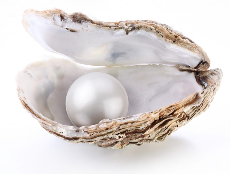
Photo via Valentyn Volkov/Shutterstock

Pearl

Unlike most gemstones that are found within the Earth, pearls have an organic origin. They are created inside the shells of certain species of oysters and clams. Some pearls are found naturally in mollusks that inhabit the sea or freshwater settings such as rivers. However, many pearls today are cultured-raised in oyster farms that sustain a thriving pearl industry. Pearls are made mostly of aragonite, a relatively soft carbonate mineral (CaCO3) that also makes up the shells of mollusks.

A pearl is created when a very small fragment of rock, a sand grain, or a parasite enters the mollusk’s shell. It irritates the oyster or clam, who responds by coating the foreign material with layer upon layer of shell material. Pearls formed on the inside of the shell are usually irregular in shape and have little commercial value. However, those formed within the tissue of the mollusk are either spherical or pear-shaped, and are highly sought out for jewelry.

Pearls possess a uniquely delicate translucence and luster that place them among the most highly valued of gemstones. The color of the pearl depends very much on the species of mollusk that produced it, and its environment. White is perhaps the best-known and most common color. However, pearls also come in delicate shades of black, cream, gray, blue, yellow, lavender, green, and mauve. Black pearls can be found in the Gulf of Mexico and waters off some islands in the Pacific Ocean. The Persian Gulf and Sri Lanka are well-known for exquisite cream-colored pearls called Orientals. Other localities for natural seawater pearls include the waters off the Celebes in Indonesia, the Gulf of California, and the Pacific coast of Mexico. The Mississippi River and forest streams of Bavaria, Germany, contain pearl-producing freshwater mussels.

Japan is famous for its cultured pearls. Everyone familiar with jewelry has heard of Mikimoto pearls, named after the creator of the industry, Kokichi Mikimoto. Cultured pearls are bred in large oyster beds in Japanese waters. An “irritant,” such as a tiny fragment of mother-of-pearl, is introduced into the fleshy part of two- to three-year-old oysters. The oysters are then grown in mesh bags submerged beneath the water and regularly fed for as long as seven to nine years before being harvested to remove their pearls. Cultured pearl industries are also carried out in Australia and equatorial islands of the Pacific.

The largest pearl in the world is believed to be about three inches long and two inches across, weighing one-third of a pound. Called the Pearl of Asia, it was a gift from Shah Jahan of India to his favorite wife, Mumtaz, for whom he also built the Taj Mahal.

La Peregrina (the Wanderer) is considered by many experts to be the most beautiful pearl. It was said to be originally found by a slave in Panama in the 1500s, who gave it up in return for his freedom. In 1570, the conquistador ruler of the area sent the pearl to King Philip II of Spain. This pear-shaped white pearl, one and a half inches in length, hangs from a platinum mount studded with diamonds. The pearl was passed to Mary I of England, then to Prince Louis Napoleon of France. He sold it to the British Marquis of Abercorn, whose family kept the pearl until 1969, when they offered it for sale at Sotheby’s. Actor Richard Burton bought it for his wife, Elizabeth Taylor.

Pearls, according to South Asian mythology, were dewdrops from heaven that fell into the sea. They were caught by shellfish under the first rays of the rising sun, during a period of full moon. In India, warriors encrusted their swords with pearls to symbolize the tears and sorrow that a sword brings.

Pearls were also widely used as medicine in Europe until the 17th century. Arabs and Persians believed it was a cure for various kinds of diseases, including insanity. Pearls have also been used as medicine as early as 2000 BC in China, where they were believed to represent wealth, power and longevity. Even to this day, lowest-grade pearls are ground for use as medicine in Asia.

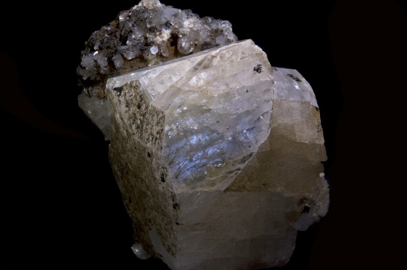
Moonstone. Image via Wikipedia

Moonstone
June’s second birthstone is the moonstone. Moonstones are believed to be named for the bluish white spots within them, that when held up to light project a silvery play of color very much like moonlight. When the stone is moved back and forth, the brilliant silvery rays appear to move about, like moonbeams playing over water.

This gemstone belongs to the family of minerals called feldspars, an important group of silicate minerals commonly formed in rocks. About half the Earth’s crust is composed of feldspar. This mineral occurs in many igneous and metamorphic rocks, and also constitutes a large percentage of soils and marine clays.

Rare geologic conditions produce gem varieties of feldspar such as moonstone, labradorite, amazonite, and sunstone. They appear as large clean mineral grains, found in pegmatites (coarse-grained igneous rock) and ancient deep crustal rocks. Feldspars of gem quality are aluminosilicates (minerals containing aluminum, silicon and oxygen), that are mixed with sodium and potassium. The best moonstones are from Sri Lanka. They are also found in the Alps, Madagascar, Myanmar (Burma), and India.

The ancient Roman natural historian, Pliny, said that the moonstone changed in appearance with the phases of the moon, a belief that persisted until the sixteenth century. The ancient Romans also believed that the image of Diana, goddess of the moon, was enclosed within the stone. Moonstones were believed to have the power to bring victory, health, and wisdom to those who wore it.

In India, the moonstone is considered a sacred stone and often displayed on a yellow cloth – yellow being considered a sacred color. The stone is believed to bring good fortune, brought on by a spirit that lives within the stone.

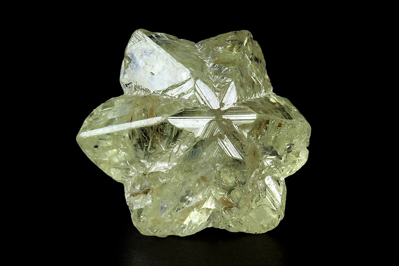
Alexandrite. Image via Wikipedia.

Alexandrite
June’s third birthstone is the alexandrite. Alexandrite possesses an enchanting chameleon-like personality. In daylight, it appears as a beautiful green, sometimes with a bluish cast or a brownish tint. However, under artificial lighting, the stone turns reddish-violet or violet.

Alexandrite belongs to the chrysoberyl family, a mineral called beryllium aluminum oxide in chemistry jargon, that contains the elements beryllium, aluminum and oxygen (BeAl2O4). It is a hard mineral, only surpassed in hardness by diamonds and corundum (sapphires and rubies). The unusual colors in alexandrite are attributed to the presence of chromium in the mineral. Chrysoberyl is found to crystallize in pegmatites (very coarse-grained igneous rock, crystallized from magma) rich in beryllium. They are also found in alluvial deposits – weathered pegmatites, containing the gemstones, that are carried by rivers and streams.

Alexandrite is an uncommon stone, and therefore very expensive. Sri Lanka is the main source of alexandrite today, and the stones have also been found in Brazil, Madagascar, Zimbabwe, Tanzania, and Myanmar (Burma). Synthetic alexandrite, resembling a reddish-hued amethyst with a tinge of green, has been manufactured but the color change seen from natural to artificial lighting cannot be reproduced. Such stones have met with only marginal market success in the United States.

The stone is named after Prince Alexander of Russia, who was to become Czar Alexander II in 1855. Discovered in 1839 on the prince’s birthday, alexandrite was found in an emerald mine in the Ural Mountains of Russia.

Because it is a relatively recent discovery, there has been little time for myth and superstition to build around this unusual stone. In Russia, the stone was also popular because it reflected the Russian national colors, green and red, and was believed to bring good luck.

Enjoying EarthSky so far? Sign up for our free daily newsletter today!

Find out about the birthstones for the other months of the year.
January birthstone
February birthstone
March birthstone
April birthstone
May birthstone
July birthstone
August birthstone
September birthstone
October birthstone
November birthstone
December birthstone

Bottom line: The month of June has 3 birthstones: Pearl, moonstone, and Alexandrite.

from EarthSky https://ift.tt/2AxIRJZ

Photo via Valentyn Volkov/Shutterstock

Pearl

Unlike most gemstones that are found within the Earth, pearls have an organic origin. They are created inside the shells of certain species of oysters and clams. Some pearls are found naturally in mollusks that inhabit the sea or freshwater settings such as rivers. However, many pearls today are cultured-raised in oyster farms that sustain a thriving pearl industry. Pearls are made mostly of aragonite, a relatively soft carbonate mineral (CaCO3) that also makes up the shells of mollusks.

A pearl is created when a very small fragment of rock, a sand grain, or a parasite enters the mollusk’s shell. It irritates the oyster or clam, who responds by coating the foreign material with layer upon layer of shell material. Pearls formed on the inside of the shell are usually irregular in shape and have little commercial value. However, those formed within the tissue of the mollusk are either spherical or pear-shaped, and are highly sought out for jewelry.

Pearls possess a uniquely delicate translucence and luster that place them among the most highly valued of gemstones. The color of the pearl depends very much on the species of mollusk that produced it, and its environment. White is perhaps the best-known and most common color. However, pearls also come in delicate shades of black, cream, gray, blue, yellow, lavender, green, and mauve. Black pearls can be found in the Gulf of Mexico and waters off some islands in the Pacific Ocean. The Persian Gulf and Sri Lanka are well-known for exquisite cream-colored pearls called Orientals. Other localities for natural seawater pearls include the waters off the Celebes in Indonesia, the Gulf of California, and the Pacific coast of Mexico. The Mississippi River and forest streams of Bavaria, Germany, contain pearl-producing freshwater mussels.

Japan is famous for its cultured pearls. Everyone familiar with jewelry has heard of Mikimoto pearls, named after the creator of the industry, Kokichi Mikimoto. Cultured pearls are bred in large oyster beds in Japanese waters. An “irritant,” such as a tiny fragment of mother-of-pearl, is introduced into the fleshy part of two- to three-year-old oysters. The oysters are then grown in mesh bags submerged beneath the water and regularly fed for as long as seven to nine years before being harvested to remove their pearls. Cultured pearl industries are also carried out in Australia and equatorial islands of the Pacific.

The largest pearl in the world is believed to be about three inches long and two inches across, weighing one-third of a pound. Called the Pearl of Asia, it was a gift from Shah Jahan of India to his favorite wife, Mumtaz, for whom he also built the Taj Mahal.

La Peregrina (the Wanderer) is considered by many experts to be the most beautiful pearl. It was said to be originally found by a slave in Panama in the 1500s, who gave it up in return for his freedom. In 1570, the conquistador ruler of the area sent the pearl to King Philip II of Spain. This pear-shaped white pearl, one and a half inches in length, hangs from a platinum mount studded with diamonds. The pearl was passed to Mary I of England, then to Prince Louis Napoleon of France. He sold it to the British Marquis of Abercorn, whose family kept the pearl until 1969, when they offered it for sale at Sotheby’s. Actor Richard Burton bought it for his wife, Elizabeth Taylor.

Pearls, according to South Asian mythology, were dewdrops from heaven that fell into the sea. They were caught by shellfish under the first rays of the rising sun, during a period of full moon. In India, warriors encrusted their swords with pearls to symbolize the tears and sorrow that a sword brings.

Pearls were also widely used as medicine in Europe until the 17th century. Arabs and Persians believed it was a cure for various kinds of diseases, including insanity. Pearls have also been used as medicine as early as 2000 BC in China, where they were believed to represent wealth, power and longevity. Even to this day, lowest-grade pearls are ground for use as medicine in Asia.

Moonstone. Image via Wikipedia

Moonstone
June’s second birthstone is the moonstone. Moonstones are believed to be named for the bluish white spots within them, that when held up to light project a silvery play of color very much like moonlight. When the stone is moved back and forth, the brilliant silvery rays appear to move about, like moonbeams playing over water.

This gemstone belongs to the family of minerals called feldspars, an important group of silicate minerals commonly formed in rocks. About half the Earth’s crust is composed of feldspar. This mineral occurs in many igneous and metamorphic rocks, and also constitutes a large percentage of soils and marine clays.

Rare geologic conditions produce gem varieties of feldspar such as moonstone, labradorite, amazonite, and sunstone. They appear as large clean mineral grains, found in pegmatites (coarse-grained igneous rock) and ancient deep crustal rocks. Feldspars of gem quality are aluminosilicates (minerals containing aluminum, silicon and oxygen), that are mixed with sodium and potassium. The best moonstones are from Sri Lanka. They are also found in the Alps, Madagascar, Myanmar (Burma), and India.

The ancient Roman natural historian, Pliny, said that the moonstone changed in appearance with the phases of the moon, a belief that persisted until the sixteenth century. The ancient Romans also believed that the image of Diana, goddess of the moon, was enclosed within the stone. Moonstones were believed to have the power to bring victory, health, and wisdom to those who wore it.

In India, the moonstone is considered a sacred stone and often displayed on a yellow cloth – yellow being considered a sacred color. The stone is believed to bring good fortune, brought on by a spirit that lives within the stone.

Alexandrite. Image via Wikipedia.

Alexandrite
June’s third birthstone is the alexandrite. Alexandrite possesses an enchanting chameleon-like personality. In daylight, it appears as a beautiful green, sometimes with a bluish cast or a brownish tint. However, under artificial lighting, the stone turns reddish-violet or violet.

Alexandrite belongs to the chrysoberyl family, a mineral called beryllium aluminum oxide in chemistry jargon, that contains the elements beryllium, aluminum and oxygen (BeAl2O4). It is a hard mineral, only surpassed in hardness by diamonds and corundum (sapphires and rubies). The unusual colors in alexandrite are attributed to the presence of chromium in the mineral. Chrysoberyl is found to crystallize in pegmatites (very coarse-grained igneous rock, crystallized from magma) rich in beryllium. They are also found in alluvial deposits – weathered pegmatites, containing the gemstones, that are carried by rivers and streams.

Alexandrite is an uncommon stone, and therefore very expensive. Sri Lanka is the main source of alexandrite today, and the stones have also been found in Brazil, Madagascar, Zimbabwe, Tanzania, and Myanmar (Burma). Synthetic alexandrite, resembling a reddish-hued amethyst with a tinge of green, has been manufactured but the color change seen from natural to artificial lighting cannot be reproduced. Such stones have met with only marginal market success in the United States.

The stone is named after Prince Alexander of Russia, who was to become Czar Alexander II in 1855. Discovered in 1839 on the prince’s birthday, alexandrite was found in an emerald mine in the Ural Mountains of Russia.

Because it is a relatively recent discovery, there has been little time for myth and superstition to build around this unusual stone. In Russia, the stone was also popular because it reflected the Russian national colors, green and red, and was believed to bring good luck.

Enjoying EarthSky so far? Sign up for our free daily newsletter today!

Find out about the birthstones for the other months of the year.
January birthstone
February birthstone
March birthstone
April birthstone
May birthstone
July birthstone
August birthstone
September birthstone
October birthstone
November birthstone
December birthstone

Bottom line: The month of June has 3 birthstones: Pearl, moonstone, and Alexandrite.

from EarthSky https://ift.tt/2AxIRJZ