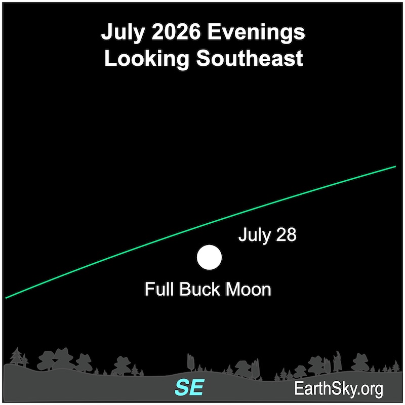
When to watch in 2026: The moment of full moon comes on July 29 for the Americas, Europe and Africa. And it falls on July 30 for Australia, New Zealand and Asia. Same full moon for all of Earth … but different time zones.
Crest of the full moon: will fall at 9:36 a.m. CDT (14:36 UTC) on July 29, 2026. That’s 2:36 a.m. New Zealand Standard Time on July 30. So, if you live in either North or South America, your fullest moon hangs low above the western horizon at sunrise on July 29. But it will also look full as it rises on the evenings of July 28 and 29.
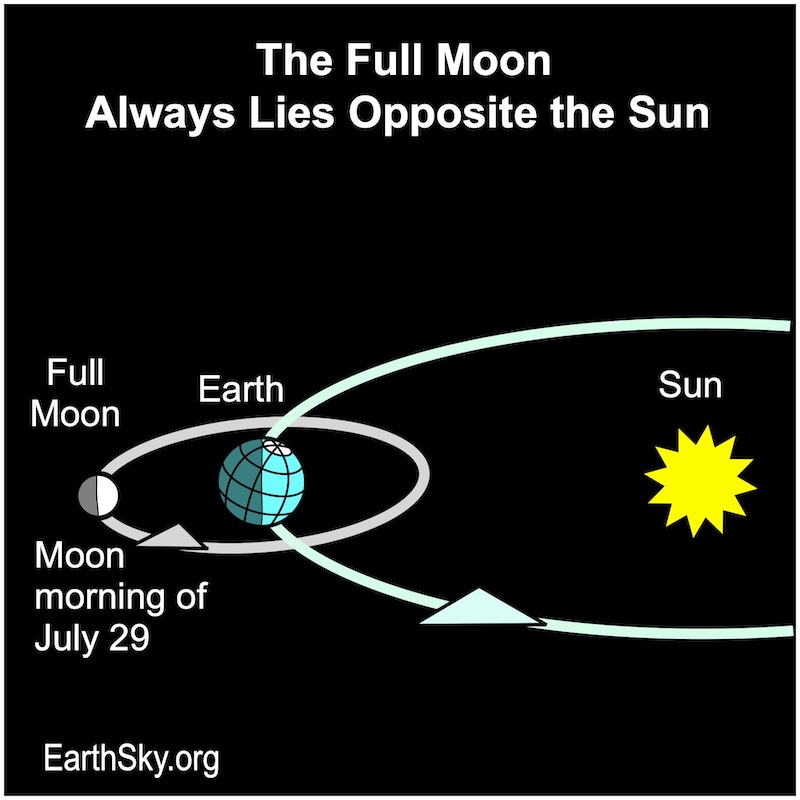
Where to look: Full moons are always opposite the sun. They must be, in order to look full. For all of us on Earth, the full moon will rise in the east just after sunset on those evenings. And it will appear highest in the sky in the middle of the night and set in the west at dawn.
July’s full moon is the Buck Moon
All the full moons have names. Popular nicknames for the July full moon include the Thunder Moon and Hay Moon … and there are lots more.
But the Buck Moon is the most common name for us in North America for the July full moon. Male deer start growing their antlers when they are about a year old. The antlers take about 120 days, or about 4 months, to mature.
By July, for us in the Northern Hemisphere, the antlers of male deer are growing fast. Sometimes they grow as fast as several inches per day. They are fully mature in fall. So, to honor the deer and the July full moon, the July full moon is the Buck Moon.
This July full moon mimics the late January sun
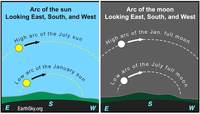
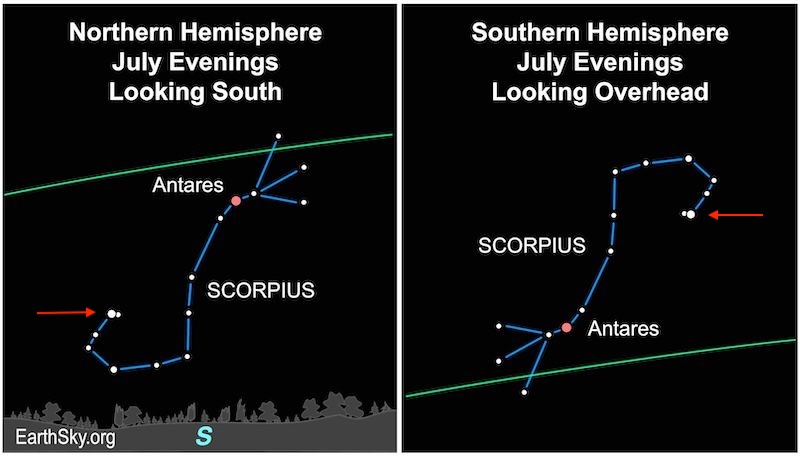
All full moons throughout the year have their own unique characteristics, often related to their paths across the sky. The full moon’s nighttime path mimics the sun’s daytime path from six months ago, or in six months from now. So, for all of us on Earth, the July full moon will follow the path the sun took in January. And, for us in the Northern Hemisphere, the January sun arched low, so we see the July full moon riding low in the sky.
In fact, in most years, again for us in the Northern Hemisphere, the path across the sky of July’s full moon is lower than any other, except the path of the full moon of June. Because it is lower, it also spends less time in the sky.
Even north of the Arctic Circle, the July full moon follows the path of the low Arctic January sun. As seen from the Arctic, the July full moon appears above the horizon only briefly. In regions closer to the North Pole, it never rises at all.
Arc of the July full moon in the Southern Hemisphere
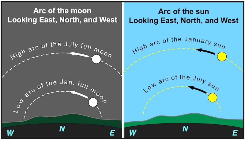
For those in the Southern Hemisphere, the July full moon’s arc across the sky matches the path of the January sun.
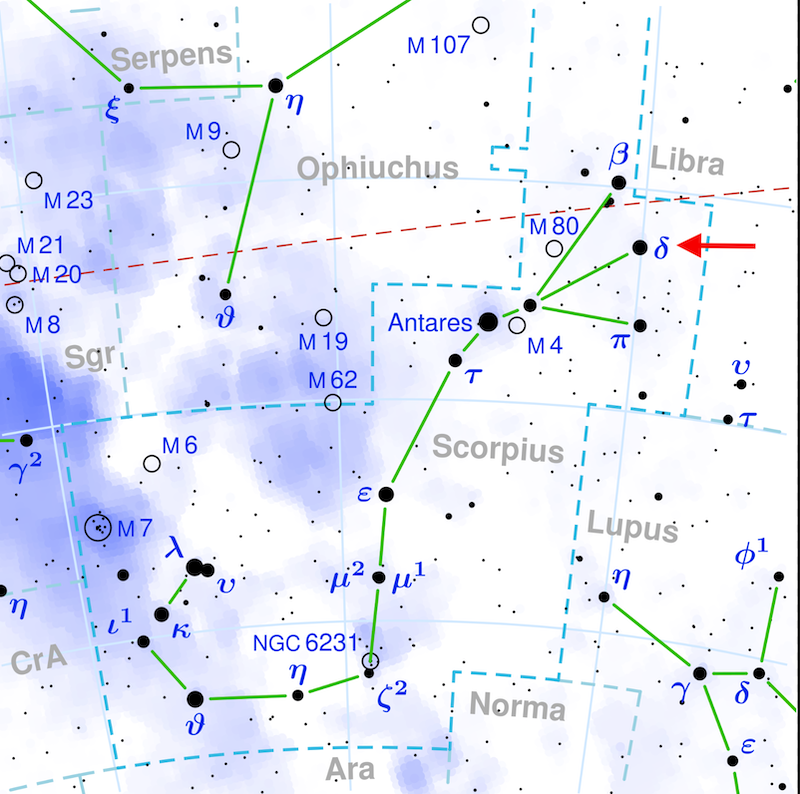
July full moon lies in Capricornus in 2026
And what of our whole-Earth perspective on the moon?
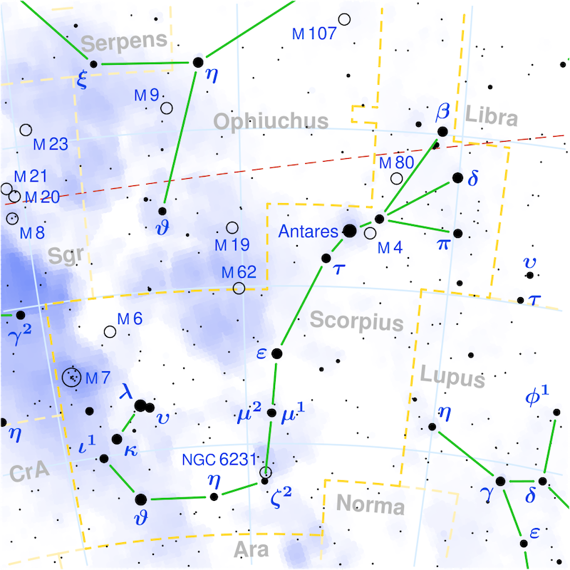
The orderliness of the heavens is such that in July the full moon always lies in front of one of two constellations of the zodiac. In most years, the July full moon appears in front of Sagittarius the Archer. This year, though, the July full moon is in front of the neighboring constellation to the east, Capricornus the Sea Goat. It is found in a dark sky in the shape of an arrowhead.
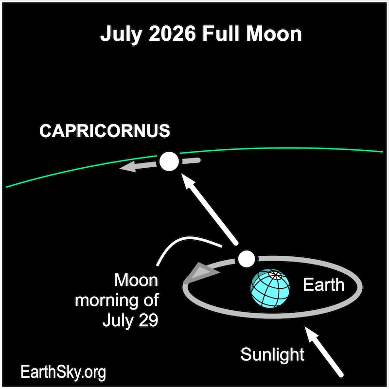
Will you recognize the arrowhead shape among the stars near the full moon? Probably not, because the full moon’s bright light will wash fainter stars from view. But you don’t need to see Capricornus’ arrowhead to know it’s there … or to know that the stars lie beyond the moon in space. As Earth orbits the sun, our planet’s night side points out on a shifting panorama of stars. And so the moon returns year after year to this quiet corner of the heavens. This is not by chance, but by the rhythms of Earth and sky.
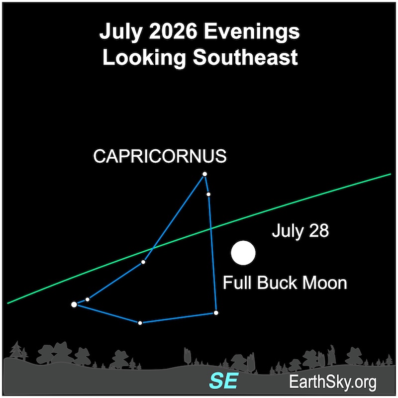
Bottom line: July’s full moon – the Buck Moon – falls on the morning of July 29, but will also appear full when it rises in the evening on July 28 and 29.
Read more: Full moon names of the month and by the season
Read more: Why do female caribou have antlers unlike other female deer?
The post The July full moon is the beautiful Buck Moon first appeared on EarthSky.
from EarthSky https://ift.tt/Ol0QLpY
When to watch in 2026: The moment of full moon comes on July 29 for the Americas, Europe and Africa. And it falls on July 30 for Australia, New Zealand and Asia. Same full moon for all of Earth … but different time zones.
Crest of the full moon: will fall at 9:36 a.m. CDT (14:36 UTC) on July 29, 2026. That’s 2:36 a.m. New Zealand Standard Time on July 30. So, if you live in either North or South America, your fullest moon hangs low above the western horizon at sunrise on July 29. But it will also look full as it rises on the evenings of July 28 and 29.
Where to look: Full moons are always opposite the sun. They must be, in order to look full. For all of us on Earth, the full moon will rise in the east just after sunset on those evenings. And it will appear highest in the sky in the middle of the night and set in the west at dawn.
July’s full moon is the Buck Moon
All the full moons have names. Popular nicknames for the July full moon include the Thunder Moon and Hay Moon … and there are lots more.
But the Buck Moon is the most common name for us in North America for the July full moon. Male deer start growing their antlers when they are about a year old. The antlers take about 120 days, or about 4 months, to mature.
By July, for us in the Northern Hemisphere, the antlers of male deer are growing fast. Sometimes they grow as fast as several inches per day. They are fully mature in fall. So, to honor the deer and the July full moon, the July full moon is the Buck Moon.
This July full moon mimics the late January sun
All full moons throughout the year have their own unique characteristics, often related to their paths across the sky. The full moon’s nighttime path mimics the sun’s daytime path from six months ago, or in six months from now. So, for all of us on Earth, the July full moon will follow the path the sun took in January. And, for us in the Northern Hemisphere, the January sun arched low, so we see the July full moon riding low in the sky.
In fact, in most years, again for us in the Northern Hemisphere, the path across the sky of July’s full moon is lower than any other, except the path of the full moon of June. Because it is lower, it also spends less time in the sky.
Even north of the Arctic Circle, the July full moon follows the path of the low Arctic January sun. As seen from the Arctic, the July full moon appears above the horizon only briefly. In regions closer to the North Pole, it never rises at all.
Arc of the July full moon in the Southern Hemisphere
For those in the Southern Hemisphere, the July full moon’s arc across the sky matches the path of the January sun.
July full moon lies in Capricornus in 2026
And what of our whole-Earth perspective on the moon?
The orderliness of the heavens is such that in July the full moon always lies in front of one of two constellations of the zodiac. In most years, the July full moon appears in front of Sagittarius the Archer. This year, though, the July full moon is in front of the neighboring constellation to the east, Capricornus the Sea Goat. It is found in a dark sky in the shape of an arrowhead.
Will you recognize the arrowhead shape among the stars near the full moon? Probably not, because the full moon’s bright light will wash fainter stars from view. But you don’t need to see Capricornus’ arrowhead to know it’s there … or to know that the stars lie beyond the moon in space. As Earth orbits the sun, our planet’s night side points out on a shifting panorama of stars. And so the moon returns year after year to this quiet corner of the heavens. This is not by chance, but by the rhythms of Earth and sky.
Bottom line: July’s full moon – the Buck Moon – falls on the morning of July 29, but will also appear full when it rises in the evening on July 28 and 29.
Read more: Full moon names of the month and by the season
Read more: Why do female caribou have antlers unlike other female deer?
The post The July full moon is the beautiful Buck Moon first appeared on EarthSky.
from EarthSky https://ift.tt/Ol0QLpY


.jpg)