Permafrost and wetland emissions could cut 1.5C carbon budget ‘by five years’

This is a re-post from Carbon Brief by Robert McSweeney

Emissions of CO2 and methane from wetlands and thawing permafrost as the climate warms could cut the “carbon budget” for the Paris Agreement temperature limits by around five years, a new study says.

These natural processes are “positive feedbacks” – so called because they release more greenhouse gases as global temperatures rise, thus reinforcing the warming. They have previously not been represented in carbon budget estimates as they are not included in most climate models, the researchers say.

The findings suggest that human-caused emissions will need to be cut by an additional 20% in order to meet the Paris Agreement’s 1.5C or 2C limits, the researchers estimate.

‘Engines for turning CO2 into methane’

Over the last year or so, there has been a flurry of new carbon budget studies – using slightly different approaches to estimate how much CO2 we can emit and still hold global temperature rise to no more than 1.5C or 2C above pre-industrial levels.

(Carbon Brief summarised all the 1.5C budgets in a recent analysis piece.)

Many of these studies use global climate models to make their estimates. However, there are some processes which affect the climate that are not yet incorporated into these models.

The new study, published in Nature Geoscience, aims to fill that gap. It focuses on two processes on the land surface: thawing permafrost and natural wetlands.

These are both positive feedbacks for the climate because, as they respond to rising temperatures, they cause the release of more greenhouse gases into the atmosphere.

Permafrost is the name given to soil that has been frozen for at least two years. It is predominantly found in the northern hemisphere – stretching across northern reaches of Russia, Canada and Alaska.

A massive permafrost thaw slump near the Arctic Ocean coastline, Canada. Credit: National Geographic Creative/Alamy Stock Photo.

These soils hold a huge amount of carbon, accumulated from dead plants and animals over thousands of years. Rising temperatures put this carbon at risk of being released, explains Dr Chris Jones, head of the earth system and mitigation science team at the Met Office Hadley Centre. Jones is not an author on the new study, but his team was involved closely in the work. He tells Carbon Brief:

“While [permafrost] is frozen, it is inert. As it thaws, this carbon is vulnerable to decomposition – like any other soil carbon. Depending on whether it is waterlogged or not this can be emitted to the atmosphere as CO2 or methane.”

How much is released as CO2 and how much as methane is still uncertain, and is an active area of research. Methane is a potent greenhouse gas – approximately 26 times more powerful than CO2 at trapping heat in the atmosphere, although it only lasts for around a decade in the atmosphere.

In natural wetlands, plants absorb CO2 from the atmosphere as they grow. But, because they are waterlogged, when the plants decompose they release methane, rather than CO2. This makes wetlands “effectively engines for turning CO2 into methane”, says Jones.

In the Amazon, for example, flooded forests actually release methane through the trees themselves.

Wetlands respond to a warming climate in three ways, Jones explains:

“As [the climate] warms, the local decomposition rate increases. Also, as rainfall changes, we may see increased or decreased areas of wetlands. This varies regionally and, again, is a large uncertainty across climate models. Finally, a direct effect of increased CO2 in the atmosphere is to increase the growth rate of the vegetation and, hence, increase the amount of CO2 being turned into methane.”

The study is the first to bring all these factors together, he notes.

Inverted model

The researchers used a “multi-layered soil carbon model” called JULES (Joint UK Land Environment Simulator), explains lead author Dr Edward Comyn-Platt, a land surface modeller at the Centre for Ecology & Hydrology. JULES has an improved representation of soil chemistry and the way that wetlands create methane.

With permafrost, for example, “this not only improves our estimates of the carbon stored in soils at high latitudes, but also allows us to estimate how much of this soil will be lost as the permafrost regions thaw”, Comyn-Platt tells Carbon Brief.

To estimate carbon budgets, the researchers use an “inverted” form of the model. This means, rather than plugging in pathways of future greenhouse gas emissions and seeing how global temperatures respond, the researchers input pathways of global temperature rise and use the model to estimate the corresponding levels of greenhouse gases in the atmosphere.

The study looks at three scenarios of future global warming: holding temperature rise at 1.5C and 2C, and one where warming “overshoots” 1.5C, reaches 1.75C, then returns to 1.5C.

In their “control” model runs with no permafrost or wetland feedbacks, the researchers estimate the 1.5C budget at 720bn-929bn tonnes of CO2 from the beginning of 2018 – equivalent to 20-25 years of emissions at current rates.

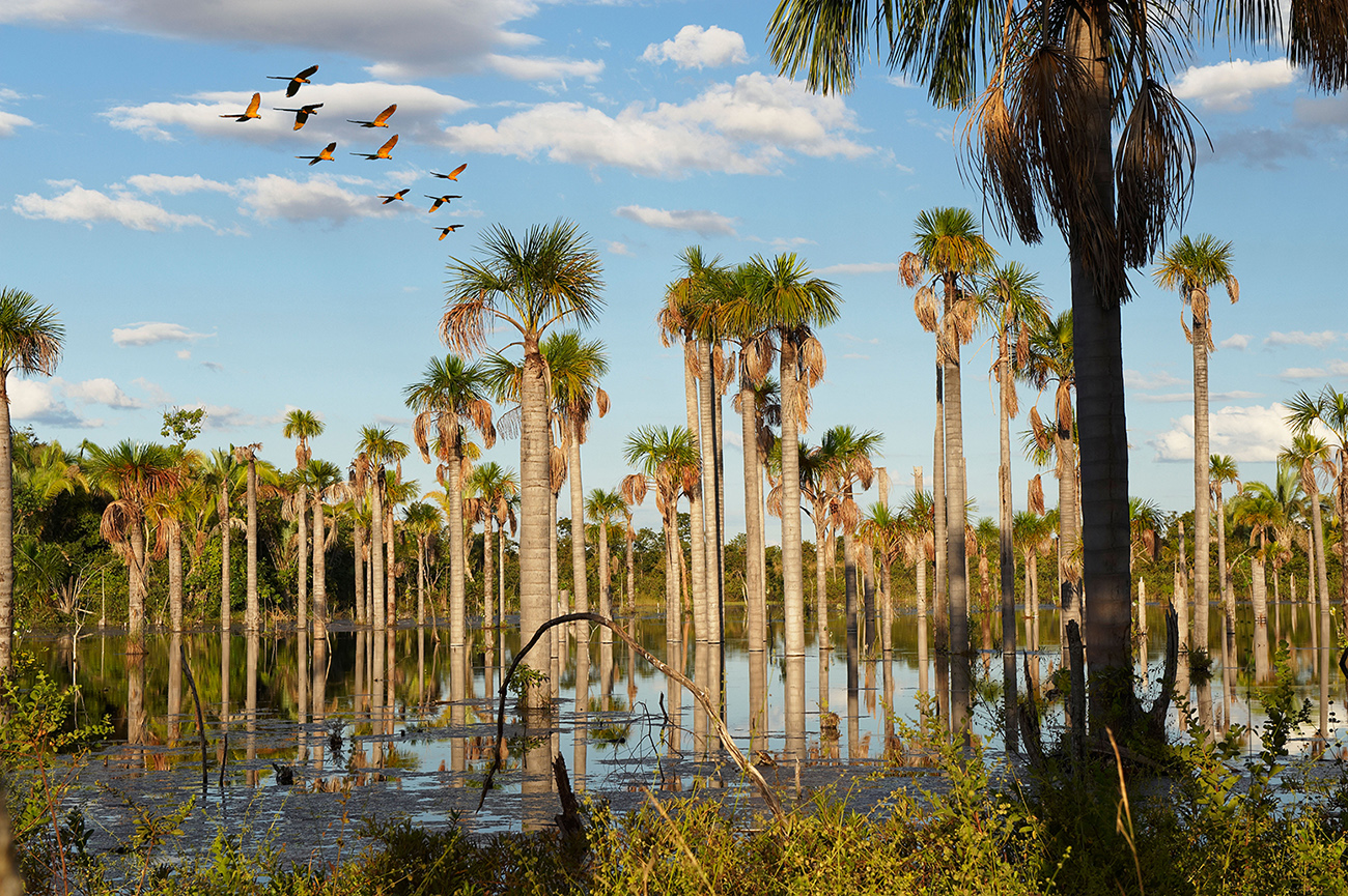
Wetlands with palms and flying blue and yellow macaws, Mato Grosso, Brazil, 2009. Credit: Juergen Ritterbach/Alamy Stock Photo.

This is slightly higher than some recent budgets because the JULES model tends to simulate a large amount of carbon uptake from the land surface, explains Comyn-Platt, freeing up space for more CO2 emissions in the budget.

The researchers then used the model to simulate the response of permafrost and natural wetlands to climate change. When the additional CO2 and methane emissions are incorporated, the available carbon budget shrinks substantially – falling to 533bn-753bn tonnes of CO2 for 1.5C, or 14-20 years of emissions.

That means accounting for the impacts of permafrost and wetlands takes around five years off the 1.5C budget. And, as the table below shows, the budgets for the 1.5C overshoot and 2C scenarios are similarly reduced.

	Control		Feedbacks included
	Tonne of CO2	Years of emissions	Tonne of CO2	Years of emissions
1.5C	720-929bn	20-25	533-753bn	14-20
1.5C overshoot	723-947bn	20-26	522-771bn	14-21
2C	1592-1974bn	43-54	1372-1776bn	37-48

Table shows remaining carbon budget (from 2018 to 2100) for three temperature pathways for the “control”  (left) and “feedbacks included” (right) scenarios. Carbon budgets are shown as tonnes of CO2 and as total years of emissions (based on 2017 global emissions). Table adapted from Comyn-Platt et al. (2018)

Evolution

This “nice work” shows that even if we were to get net emissions to zero in the next few decades, emissions would need to fall further in order to stabilise temperatures at 1.5C or 2C, says Prof Piers Forster, professor of physical climate change at the University of Leeds and director of the Priestley International Centre for Climate. He tells Carbon Brief:

“The extra carbon released from thawing permafrost and warming wetlands would continue beyond the date of net-zero emissions and this would need to be countered for in order to consider carbon budgets applicable for 2100 and beyond.”

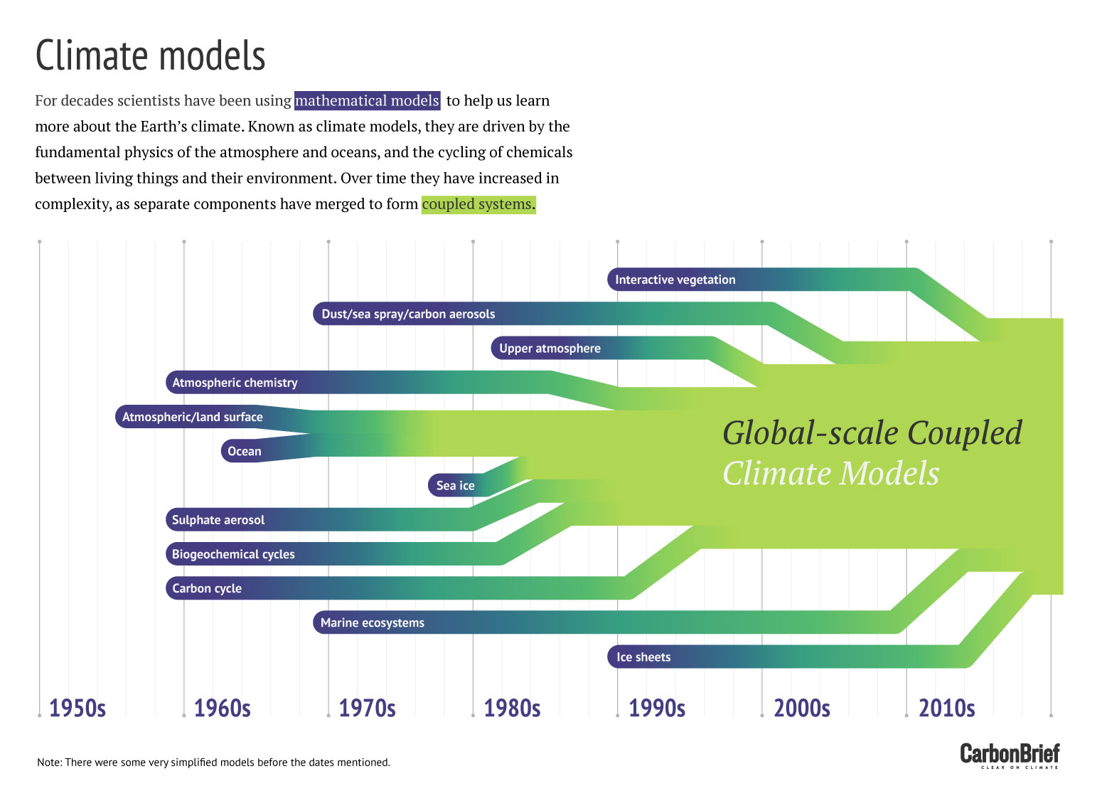
The study also highlights the constant evolution in the complexity of climate models, says Jones, with new model components being developed and run separately before being incorporated into global models.

The graphic below shows how new components have been added to global climate models over time.

In this case, the wetland model “scheme” will be shortly be brought into UKESM1 – the UK Earth System Model run by the Met Office Hadley Centre and partners, says Jones. And the permafrost scheme “will follow in due course”.

 

Comyn-Platt, E. et al. (2018) Carbon budgets for 1.5 and 2C targets lowered by natural wetland and permafrost feedbacks, Nature Geoscience, doi:10.1038/s41561-018-0174-9 

 

from Skeptical Science https://ift.tt/2LUMLkl

This is a re-post from Carbon Brief by Robert McSweeney

Emissions of CO2 and methane from wetlands and thawing permafrost as the climate warms could cut the “carbon budget” for the Paris Agreement temperature limits by around five years, a new study says.

These natural processes are “positive feedbacks” – so called because they release more greenhouse gases as global temperatures rise, thus reinforcing the warming. They have previously not been represented in carbon budget estimates as they are not included in most climate models, the researchers say.

The findings suggest that human-caused emissions will need to be cut by an additional 20% in order to meet the Paris Agreement’s 1.5C or 2C limits, the researchers estimate.

‘Engines for turning CO2 into methane’

Over the last year or so, there has been a flurry of new carbon budget studies – using slightly different approaches to estimate how much CO2 we can emit and still hold global temperature rise to no more than 1.5C or 2C above pre-industrial levels.

(Carbon Brief summarised all the 1.5C budgets in a recent analysis piece.)

Many of these studies use global climate models to make their estimates. However, there are some processes which affect the climate that are not yet incorporated into these models.

The new study, published in Nature Geoscience, aims to fill that gap. It focuses on two processes on the land surface: thawing permafrost and natural wetlands.

These are both positive feedbacks for the climate because, as they respond to rising temperatures, they cause the release of more greenhouse gases into the atmosphere.

Permafrost is the name given to soil that has been frozen for at least two years. It is predominantly found in the northern hemisphere – stretching across northern reaches of Russia, Canada and Alaska.

A massive permafrost thaw slump near the Arctic Ocean coastline, Canada. Credit: National Geographic Creative/Alamy Stock Photo.

These soils hold a huge amount of carbon, accumulated from dead plants and animals over thousands of years. Rising temperatures put this carbon at risk of being released, explains Dr Chris Jones, head of the earth system and mitigation science team at the Met Office Hadley Centre. Jones is not an author on the new study, but his team was involved closely in the work. He tells Carbon Brief:

“While [permafrost] is frozen, it is inert. As it thaws, this carbon is vulnerable to decomposition – like any other soil carbon. Depending on whether it is waterlogged or not this can be emitted to the atmosphere as CO2 or methane.”

How much is released as CO2 and how much as methane is still uncertain, and is an active area of research. Methane is a potent greenhouse gas – approximately 26 times more powerful than CO2 at trapping heat in the atmosphere, although it only lasts for around a decade in the atmosphere.

In natural wetlands, plants absorb CO2 from the atmosphere as they grow. But, because they are waterlogged, when the plants decompose they release methane, rather than CO2. This makes wetlands “effectively engines for turning CO2 into methane”, says Jones.

In the Amazon, for example, flooded forests actually release methane through the trees themselves.

Wetlands respond to a warming climate in three ways, Jones explains:

“As [the climate] warms, the local decomposition rate increases. Also, as rainfall changes, we may see increased or decreased areas of wetlands. This varies regionally and, again, is a large uncertainty across climate models. Finally, a direct effect of increased CO2 in the atmosphere is to increase the growth rate of the vegetation and, hence, increase the amount of CO2 being turned into methane.”

The study is the first to bring all these factors together, he notes.

Inverted model

The researchers used a “multi-layered soil carbon model” called JULES (Joint UK Land Environment Simulator), explains lead author Dr Edward Comyn-Platt, a land surface modeller at the Centre for Ecology & Hydrology. JULES has an improved representation of soil chemistry and the way that wetlands create methane.

With permafrost, for example, “this not only improves our estimates of the carbon stored in soils at high latitudes, but also allows us to estimate how much of this soil will be lost as the permafrost regions thaw”, Comyn-Platt tells Carbon Brief.

To estimate carbon budgets, the researchers use an “inverted” form of the model. This means, rather than plugging in pathways of future greenhouse gas emissions and seeing how global temperatures respond, the researchers input pathways of global temperature rise and use the model to estimate the corresponding levels of greenhouse gases in the atmosphere.

The study looks at three scenarios of future global warming: holding temperature rise at 1.5C and 2C, and one where warming “overshoots” 1.5C, reaches 1.75C, then returns to 1.5C.

In their “control” model runs with no permafrost or wetland feedbacks, the researchers estimate the 1.5C budget at 720bn-929bn tonnes of CO2 from the beginning of 2018 – equivalent to 20-25 years of emissions at current rates.

Wetlands with palms and flying blue and yellow macaws, Mato Grosso, Brazil, 2009. Credit: Juergen Ritterbach/Alamy Stock Photo.

This is slightly higher than some recent budgets because the JULES model tends to simulate a large amount of carbon uptake from the land surface, explains Comyn-Platt, freeing up space for more CO2 emissions in the budget.

The researchers then used the model to simulate the response of permafrost and natural wetlands to climate change. When the additional CO2 and methane emissions are incorporated, the available carbon budget shrinks substantially – falling to 533bn-753bn tonnes of CO2 for 1.5C, or 14-20 years of emissions.

That means accounting for the impacts of permafrost and wetlands takes around five years off the 1.5C budget. And, as the table below shows, the budgets for the 1.5C overshoot and 2C scenarios are similarly reduced.

	Control		Feedbacks included
	Tonne of CO2	Years of emissions	Tonne of CO2	Years of emissions
1.5C	720-929bn	20-25	533-753bn	14-20
1.5C overshoot	723-947bn	20-26	522-771bn	14-21
2C	1592-1974bn	43-54	1372-1776bn	37-48

Table shows remaining carbon budget (from 2018 to 2100) for three temperature pathways for the “control”  (left) and “feedbacks included” (right) scenarios. Carbon budgets are shown as tonnes of CO2 and as total years of emissions (based on 2017 global emissions). Table adapted from Comyn-Platt et al. (2018)

Evolution

This “nice work” shows that even if we were to get net emissions to zero in the next few decades, emissions would need to fall further in order to stabilise temperatures at 1.5C or 2C, says Prof Piers Forster, professor of physical climate change at the University of Leeds and director of the Priestley International Centre for Climate. He tells Carbon Brief:

“The extra carbon released from thawing permafrost and warming wetlands would continue beyond the date of net-zero emissions and this would need to be countered for in order to consider carbon budgets applicable for 2100 and beyond.”

The study also highlights the constant evolution in the complexity of climate models, says Jones, with new model components being developed and run separately before being incorporated into global models.

The graphic below shows how new components have been added to global climate models over time.

In this case, the wetland model “scheme” will be shortly be brought into UKESM1 – the UK Earth System Model run by the Met Office Hadley Centre and partners, says Jones. And the permafrost scheme “will follow in due course”.

 

Comyn-Platt, E. et al. (2018) Carbon budgets for 1.5 and 2C targets lowered by natural wetland and permafrost feedbacks, Nature Geoscience, doi:10.1038/s41561-018-0174-9 

 

from Skeptical Science https://ift.tt/2LUMLkl

New research, July 2-29, 2018

A selection of new climate related research articles is shown below.

Climate change mitigation

Climate change communication

Place, proximity, and perceived harm: extreme weather events and views about climate change

Teaching climate change in middle schools and high schools: investigating STEM education’s deficit model

Cool dudes in Norway: climate change denial among conservative Norwegian men

Emission savings

How important are future marine and shipping aerosol emissions in a warming Arctic summer and autumn? (open access)

Work time reduction and economic democracy as climate change mitigation strategies: or why the climate needs a renewed labor movement

The remaining potential for energy savings in UK households

Energy production

The slow expansion of renewable energy in Russia: Competitiveness and regulation issues

Promises and limitations of nuclear fission energy in combating climate change

Russia's Nuclear Export Programme

Better late than never, but never late is better: Risk assessment of nuclear power construction projects

The changing risk perception towards nuclear power in China after the Fukushima nuclear accident in Japan

Analyzing the factors that influence U.S. public support for exporting natural gas

Climate Policy

US and international climate policy under President Trump

The withdrawal of the U.S. from the Paris Agreement and its impact on global climate change governance (open access)

U.S. withdrawal from the Paris Agreement: Reasons, impacts, and China's response (open access)

The impacts of U.S. withdrawal from the Paris Agreement on the carbon emission space and mitigation cost of China, EU, and Japan under the constraints of the global carbon emission space (open access)

The climate lobby: a sectoral analysis of lobbying spending on climate change in the USA, 2000 to 2016

Short term policies to keep the door open for Paris climate goals (open access)

Is India pulling its weight? India’s nationally determined contribution and future energy plans in global climate policy

Climate change

Temperature, precipitation, wind

Arctic amplification metrics

Can an ensemble climate simulation be used to separate climate change signals from internal unforced variability? (open access)

Changes in surface air temperature over China under the 1.5 and 2.0 °C global warming targets (open access)

Recent subsurface North Atlantic cooling trend in context of Atlantic decadal-to-multidecadal variability (open access)

Multidecadal Changes of the Upper Indian Ocean Heat Content during 1965-2016

Detectable impacts of the past half‐degree global warming on summertime hot extremes in China

Human contribution to the increasing summer precipitation in Central Asia from 1961 to 2013

Diminishing Arctic Sea Ice Promotes Stronger Surface Winds

Extreme events

Spatiotemporal variability of tornadoes in the Czech Lands, 1801–2017

Drivers of 2016 record Arctic warmth assessed using climate simulations subjected to Factual and Counterfactual forcing (open access)

Increase in extreme precipitation events under anthropogenic warming in India (open access)

Forcings and feedbacks

Self‐amplifying feedbacks accelerate greening and warming of the Arctic

Contributions of Internal Variability and External Forcing to the Recent Pacific Decadal Variations

Assessment of the Impact of Solar Spectral Irradiance on Near‐Infrared Clear‐Sky Atmospheric Absorption and Heating Rates

Cryosphere

Ocean‐induced melt triggers glacier retreat in Northwest Greenland

Greenland Ice Mapping Project: ice flow velocity variation at sub-monthly to decadal timescales (open access)

Dynamic response of Antarctic Peninsula Ice Sheet to potential collapse of Larsen C and George VI ice shelves (open access)

Glacier change along West Antarctica's Marie Byrd Land Sector and links to inter-decadal atmosphere–ocean variability (open access)

Attribution of Arctic sea ice decline from 1953 to 2012 to influences from natural, greenhouse-gas and anthropogenic aerosol forcing

Evolution of the global coupled climate response to Arctic sea ice loss during 1990-2090 and its contribution to climate change

Responses and changes in the permafrost and snow water equivalent in the Northern Hemisphere under a scenario of 1.5 °C warming (open access)

Global snow zone maps and trends in snow persistence 2001–2016

Hydrosphere 

Rising Oceans Guaranteed: Arctic Land Ice Loss and Sea Level Rise (open access)

Sensitivity of streamflow to climate change in California

Atmospheric and oceanic circulation

Blocking and its Response to Climate Change (open access)

Two AMOC states in response to decreasing greenhouse gas concentrations in the coupled climate model MPI-ESM

Carbon cycle

Long-term response of oceanic carbon uptake to global warming via physical and biological pumps (open access)

Grasslands may be more reliable carbon sinks than forests in California (open access)

Climate change impacts

Mankind

Projected heat stress under 1.5oC and 2oC global warming scenarios creates unprecedented discomfort for humans in West Africa (open access)

Climatic variability and dengue risk in urban environment of Delhi (India)

Unprecedented risk of spring frost damage in Switzerland and Germany in 2017

Heat in the Heartland: Crop Yield and Coverage Response to Climate Change Along the Mississippi River

Economically robust protection against 21st century sea-level rise

Limits to growth redux: A system dynamics model for assessing energy and climate change constraints to global growth

Biosphere

Acceleration of global vegetation greenup from combined effects of climate change and human land management

Dramatic loss of seagrass habitat under projected climate change in the Mediterranean Sea

The Arctic picoeukaryote Micromonas pusilla benefits synergistically from warming and ocean acidification (open access)

Increasing temperature sensitivity caused by climate warming, evidence from Northeastern China

Increased growth of Qinghai spruce in northwestern China during the recent warming hiatus

Development and analysis of spring plant phenology products: 36 years of 1-km grids over the conterminous US

Impacts of recent climate extremes on spring phenology in arid-mountain ecosystems in China

Unchanged risk of frost exposure for subalpine and alpine plants after snowmelt in Switzerland despite climate warming

Effects of ocean acidification on algae growth and feeding rates of juvenile sea urchins

Transgenerational deleterious effects of ocean acidification on the reproductive success of a keystone crustacean (Gammarus locusta)

Climate change alterations to ecosystem dominance: how might sponge‐dominated reefs function?

Ecophysiological plasticity of Amazonian trees to long-term drought

Does sexual dimorphism predispose dioecious riparian trees to sex ratio imbalances under climate change?

Interactions between rising CO2 and temperature drive accelerated flowering in model plants under changing conditions of the last century

Elevated atmospheric concentrations of carbon dioxide reduce monarch tolerance and increase parasite virulence by altering the medicinal properties of milkweeds

Oysters and eelgrass: potential partners in a high pCO2 ocean

Other papers

General climate science

Understanding weather and climate of the last 300 years from ships' logbooks

Climate history of Russia and the Soviet Union

Palaeoclimatology

Large-scale, millennial-length temperature reconstructions from tree-rings

Tracing winter temperatures over the last two millennia using a north-east Atlantic coastal record (open access)

from Skeptical Science https://ift.tt/2MgIwMO

A selection of new climate related research articles is shown below.

Climate change mitigation

Climate change communication

Place, proximity, and perceived harm: extreme weather events and views about climate change

Teaching climate change in middle schools and high schools: investigating STEM education’s deficit model

Cool dudes in Norway: climate change denial among conservative Norwegian men

Emission savings

How important are future marine and shipping aerosol emissions in a warming Arctic summer and autumn? (open access)

Work time reduction and economic democracy as climate change mitigation strategies: or why the climate needs a renewed labor movement

The remaining potential for energy savings in UK households

Energy production

The slow expansion of renewable energy in Russia: Competitiveness and regulation issues

Promises and limitations of nuclear fission energy in combating climate change

Russia's Nuclear Export Programme

Better late than never, but never late is better: Risk assessment of nuclear power construction projects

The changing risk perception towards nuclear power in China after the Fukushima nuclear accident in Japan

Analyzing the factors that influence U.S. public support for exporting natural gas

Climate Policy

US and international climate policy under President Trump

The withdrawal of the U.S. from the Paris Agreement and its impact on global climate change governance (open access)

U.S. withdrawal from the Paris Agreement: Reasons, impacts, and China's response (open access)

The impacts of U.S. withdrawal from the Paris Agreement on the carbon emission space and mitigation cost of China, EU, and Japan under the constraints of the global carbon emission space (open access)

The climate lobby: a sectoral analysis of lobbying spending on climate change in the USA, 2000 to 2016

Short term policies to keep the door open for Paris climate goals (open access)

Is India pulling its weight? India’s nationally determined contribution and future energy plans in global climate policy

Climate change

Temperature, precipitation, wind

Arctic amplification metrics

Can an ensemble climate simulation be used to separate climate change signals from internal unforced variability? (open access)

Changes in surface air temperature over China under the 1.5 and 2.0 °C global warming targets (open access)

Recent subsurface North Atlantic cooling trend in context of Atlantic decadal-to-multidecadal variability (open access)

Multidecadal Changes of the Upper Indian Ocean Heat Content during 1965-2016

Detectable impacts of the past half‐degree global warming on summertime hot extremes in China

Human contribution to the increasing summer precipitation in Central Asia from 1961 to 2013

Diminishing Arctic Sea Ice Promotes Stronger Surface Winds

Extreme events

Spatiotemporal variability of tornadoes in the Czech Lands, 1801–2017

Drivers of 2016 record Arctic warmth assessed using climate simulations subjected to Factual and Counterfactual forcing (open access)

Increase in extreme precipitation events under anthropogenic warming in India (open access)

Forcings and feedbacks

Self‐amplifying feedbacks accelerate greening and warming of the Arctic

Contributions of Internal Variability and External Forcing to the Recent Pacific Decadal Variations

Assessment of the Impact of Solar Spectral Irradiance on Near‐Infrared Clear‐Sky Atmospheric Absorption and Heating Rates

Cryosphere

Ocean‐induced melt triggers glacier retreat in Northwest Greenland

Greenland Ice Mapping Project: ice flow velocity variation at sub-monthly to decadal timescales (open access)

Dynamic response of Antarctic Peninsula Ice Sheet to potential collapse of Larsen C and George VI ice shelves (open access)

Glacier change along West Antarctica's Marie Byrd Land Sector and links to inter-decadal atmosphere–ocean variability (open access)

Attribution of Arctic sea ice decline from 1953 to 2012 to influences from natural, greenhouse-gas and anthropogenic aerosol forcing

Evolution of the global coupled climate response to Arctic sea ice loss during 1990-2090 and its contribution to climate change

Responses and changes in the permafrost and snow water equivalent in the Northern Hemisphere under a scenario of 1.5 °C warming (open access)

Global snow zone maps and trends in snow persistence 2001–2016

Hydrosphere 

Rising Oceans Guaranteed: Arctic Land Ice Loss and Sea Level Rise (open access)

Sensitivity of streamflow to climate change in California

Atmospheric and oceanic circulation

Blocking and its Response to Climate Change (open access)

Two AMOC states in response to decreasing greenhouse gas concentrations in the coupled climate model MPI-ESM

Carbon cycle

Long-term response of oceanic carbon uptake to global warming via physical and biological pumps (open access)

Grasslands may be more reliable carbon sinks than forests in California (open access)

Climate change impacts

Mankind

Projected heat stress under 1.5oC and 2oC global warming scenarios creates unprecedented discomfort for humans in West Africa (open access)

Climatic variability and dengue risk in urban environment of Delhi (India)

Unprecedented risk of spring frost damage in Switzerland and Germany in 2017

Heat in the Heartland: Crop Yield and Coverage Response to Climate Change Along the Mississippi River

Economically robust protection against 21st century sea-level rise

Limits to growth redux: A system dynamics model for assessing energy and climate change constraints to global growth

Biosphere

Acceleration of global vegetation greenup from combined effects of climate change and human land management

Dramatic loss of seagrass habitat under projected climate change in the Mediterranean Sea

The Arctic picoeukaryote Micromonas pusilla benefits synergistically from warming and ocean acidification (open access)

Increasing temperature sensitivity caused by climate warming, evidence from Northeastern China

Increased growth of Qinghai spruce in northwestern China during the recent warming hiatus

Development and analysis of spring plant phenology products: 36 years of 1-km grids over the conterminous US

Impacts of recent climate extremes on spring phenology in arid-mountain ecosystems in China

Unchanged risk of frost exposure for subalpine and alpine plants after snowmelt in Switzerland despite climate warming

Effects of ocean acidification on algae growth and feeding rates of juvenile sea urchins

Transgenerational deleterious effects of ocean acidification on the reproductive success of a keystone crustacean (Gammarus locusta)

Climate change alterations to ecosystem dominance: how might sponge‐dominated reefs function?

Ecophysiological plasticity of Amazonian trees to long-term drought

Does sexual dimorphism predispose dioecious riparian trees to sex ratio imbalances under climate change?

Interactions between rising CO2 and temperature drive accelerated flowering in model plants under changing conditions of the last century

Elevated atmospheric concentrations of carbon dioxide reduce monarch tolerance and increase parasite virulence by altering the medicinal properties of milkweeds

Oysters and eelgrass: potential partners in a high pCO2 ocean

Other papers

General climate science

Understanding weather and climate of the last 300 years from ships' logbooks

Climate history of Russia and the Soviet Union

Palaeoclimatology

Large-scale, millennial-length temperature reconstructions from tree-rings

Tracing winter temperatures over the last two millennia using a north-east Atlantic coastal record (open access)

from Skeptical Science https://ift.tt/2MgIwMO

Find the Teapot, and the galaxy’s center

Tonight, or on any moonless evening during a Northern Hemisphere summer or Southern Hemisphere winter, you can look in the evening hours toward the center of our Milky Way galaxy. It’s located in the direction of Sagittarius the Archer, with happens to contain a famous asterism – or noticeable pattern of stars – called the Teapot.

From the Northern Hemisphere, you’ll be looking south during the evening hours for this star pattern. From the Southern Hemisphere, look for the Teapot to climb high overhead around mid-to-late evening.

If you’re blessed with a dark sky, finding all this will be easy. In a dark sky, you’ll see a broad boulevard of stars – the edgewise view into our own Milky Way galaxy – which broadens and brightens in the direction of the galaxy’s center.

Or maybe you know the planets? If you have that dark sky, know that, in 2018, the starry band of the Milky Way passes between the Teapot and the golden planet Saturn. It lies about midway between the spout of the Teapot and Saturn this year.

Don’t know Saturn and don’t have a dark sky? The chart below via AstroBob expands the view to include the constellation Scorpius, which is relatively bright and easy to spot for its curved Scorpion’s Tail. Sagittarius the Archer – and its Teapot asterism – is next door to Scorpius on the sky’s dome.

From the Northern Hemisphere, look southward in July and August evenings to see these stars. From the Southern Hemisphere, look generally northward, higher in the sky and turn this chart upside down. Chart via AstroBob.

We can’t really see the galactic center. It’s heavily veiled by intervening stars, star clusters and nebulae (vast clouds of gas and dust). The center of our Milky Way looms some 26,000 light-years away. But we can gaze toward this direction in space, and – if your sky is dark enough – it’s a sight to behold!

By the way, the Teapot makes up the western half of the constellation Sagittarius the Archer. Modern eyes have an easier time envisioning a teapot than an Archer with a drawn-out bow. See the sky chart of Sagittarius below.

View larger. | The constellation Sagittarius, with the Teapot asterism outlined in green.

From temperate latitudes in the Northern Hemisphere, it’s pretty easy to make out the Summer Triangle asterism rather high in the eastern sky at nightfall. This huge star formation consists of three brilliant stars – Vega, Deneb and Altair – and can oftentimes withstand the glare of the full moon or light-polluted city.

If you are otherwise lost on some starry night but can find the Summer Triangle, let this signpost star formation escort you to the Teapot …

Draw an imaginary line from Deneb through Altair to star-hop to the Teapot of Sagittarius.

Bottom line: Blessed with a dark sky? Try finding the Teapot in Sagittarius.

Read more: Sagittarius? Here’s your constellation

from EarthSky https://ift.tt/2tLSE6j

Tonight, or on any moonless evening during a Northern Hemisphere summer or Southern Hemisphere winter, you can look in the evening hours toward the center of our Milky Way galaxy. It’s located in the direction of Sagittarius the Archer, with happens to contain a famous asterism – or noticeable pattern of stars – called the Teapot.

From the Northern Hemisphere, you’ll be looking south during the evening hours for this star pattern. From the Southern Hemisphere, look for the Teapot to climb high overhead around mid-to-late evening.

If you’re blessed with a dark sky, finding all this will be easy. In a dark sky, you’ll see a broad boulevard of stars – the edgewise view into our own Milky Way galaxy – which broadens and brightens in the direction of the galaxy’s center.

Or maybe you know the planets? If you have that dark sky, know that, in 2018, the starry band of the Milky Way passes between the Teapot and the golden planet Saturn. It lies about midway between the spout of the Teapot and Saturn this year.

Don’t know Saturn and don’t have a dark sky? The chart below via AstroBob expands the view to include the constellation Scorpius, which is relatively bright and easy to spot for its curved Scorpion’s Tail. Sagittarius the Archer – and its Teapot asterism – is next door to Scorpius on the sky’s dome.

From the Northern Hemisphere, look southward in July and August evenings to see these stars. From the Southern Hemisphere, look generally northward, higher in the sky and turn this chart upside down. Chart via AstroBob.

We can’t really see the galactic center. It’s heavily veiled by intervening stars, star clusters and nebulae (vast clouds of gas and dust). The center of our Milky Way looms some 26,000 light-years away. But we can gaze toward this direction in space, and – if your sky is dark enough – it’s a sight to behold!

By the way, the Teapot makes up the western half of the constellation Sagittarius the Archer. Modern eyes have an easier time envisioning a teapot than an Archer with a drawn-out bow. See the sky chart of Sagittarius below.

View larger. | The constellation Sagittarius, with the Teapot asterism outlined in green.

From temperate latitudes in the Northern Hemisphere, it’s pretty easy to make out the Summer Triangle asterism rather high in the eastern sky at nightfall. This huge star formation consists of three brilliant stars – Vega, Deneb and Altair – and can oftentimes withstand the glare of the full moon or light-polluted city.

If you are otherwise lost on some starry night but can find the Summer Triangle, let this signpost star formation escort you to the Teapot …

Draw an imaginary line from Deneb through Altair to star-hop to the Teapot of Sagittarius.

Bottom line: Blessed with a dark sky? Try finding the Teapot in Sagittarius.

Read more: Sagittarius? Here’s your constellation

from EarthSky https://ift.tt/2tLSE6j

Living with a brain tumour – Sue’s story

Brain tumours are hard to treat and survival remains stubbornly low. That’s why brain tumour research is one of our top priorities. In the final of a 3-part series, Sue shares what it’s like to live with a brain tumour.

It might sound strange, but I was first diagnosed with a brain tumour because my gynaecologist referred me to an anaesthetist that he knew. I was 36 at the time and I’d been having migraines for years. I’d been to the GP but nothing they prescribed worked.

Botox was just coming out for migraines, but because of my medical history the anaesthetist couldn’t give me the injections without sending me for a brain scan first. That’s when they found the tumour.

I was referred to a neurosurgeon and was back in hospital within three days as an urgent case. The surgeon said he couldn’t do a biopsy because of the tumour’s location, as it would cause a massive bleed in my brain. I was straight in for surgery, which lasted five and a half hours. When my results came back, they’d found it was a grade 2 astrocytoma.

An invisible illness

Even though I’d been having symptoms for years, the diagnosis still came as a shock. I had 3 young children at the time and had to stop and think about them, and what would happen if something happened to me.

Because it wasn’t something you could see, like a broken leg, people just assumed that I was OK.

I recovered well from my operation and once I’d had my staples out and my hair was back to normal, you’d have never known I’d had brain tumour surgery.

Because it wasn’t something you could see, like a broken leg, people just assumed that I was OK now, so I didn’t feel that I got the support I needed. I wished people would have offered to take the kids out to the park for a few hours; my youngest was only 2 at the time so it was really difficult. But they just didn’t understand, which was frustrating.

At times like this you really find out who your friends are. We had some friends who, when I was on treatment, would come around and cook for us so many times. I never asked. It was brilliant, and just what I needed.

Living with unknowns

For the next 6 years I was well, and life was normal. I had to have scans every 6 months which were always OK. I don’t mind the machines, and there’s a lot to be said for building up relationships with the staff. I got to know them all and they’re all brilliant.

Then, in 2013, I had a serious seizure in my sleep while on holiday. We came back home the next day and I was given another MRI scan, but everything was fine. So, I was put on anti-seizure medication and for the next 6 months I was fine, the drugs seemed to stop everything. But then the seizures returned, first occasionally and then several times a day. The MRI scans still didn’t show anything, so in May the following year I had a different type of scan called an MRS, which is much longer and more detailed.

That picked up unusual levels of brain activity, so I had to go back in for surgery. The tumour had come back, but because it was picked up early it hadn’t had time to grow into a large mass. This time though, the tumour had changed to a grade 3.

For my type of tumour, it will never be: “You’re better now.” There’s no cure for it.

I needed to have 18 cycles of the chemotherapy drug temozolomide. It was 3 weeks on and 1 off, 18 times. It was a long, tough process. I did really well, I think it’s a brilliant drug. For me though, the worst part was the fatigue.

It really does wipe you out. But I had to carry on, and I was getting up every day to make sandwiches for my kids to take to school.

Right now, everything is OK. But for my type of tumour, it will never be: “You’re better now.” When I last saw my doctor, and asked him what my chances are, he said that unfortunately my tumour is the kind that will simmer away, and it will come back again.

There’s no cure for it. It’s how long I’ve got that’s the difficult thing to come to terms with.

For me it could be 10 years, or it could be 6 months. That’s the sad thing, I just don’t know. And that’s the way I must live.

Taking life as it comes

It’s been 11 years since my diagnosis, and I have good days and bad days. It’s changed my personality, which is probably because the tumour is near my temporal lobe, where emotions are made.

It depends on the circumstances as to how I react to people in different situations, but I’ve got a really bad temper. I know I’ve changed, but I never use the tumour as an excuse.

You’ve got to make the most of what you’ve got and enjoy the life that you have.

It’s worse when people around me have died because of their brain tumours. Because I’ve had cancer for a long time now, I’ve met a lot of people who have also had brain tumours. Some of these people haven’t been as unwell as I have, but then they’ve suddenly died from their disease, while for others their treatment hasn’t worked or stopped working.

In the last 3 months, 3 of my friends with the same tumour have had their disease come back and they didn’t have any symptoms. There just aren’t enough success stories for brain tumours.

I still have scans every 3 months, but my attitude is that I can’t change anything and I must take each day as it comes.

I’m quite tough, so I don’t believe in sitting around feeling sorry for myself. I don’t look at life as time I’ve got left. You’ve got to make the most of what you’ve got and enjoy the life that you have, because it passes you by.

If you’ve been affected by cancer and would like to speak to someone, you can call our nurses on freephone 0808 800 4040, 9am until 5pm Monday to Friday. Alternatively, you can join our friendly and supportive discussion forum, Cancer Chat.

from Cancer Research UK – Science blog https://ift.tt/2OCdOz8

Brain tumours are hard to treat and survival remains stubbornly low. That’s why brain tumour research is one of our top priorities. In the final of a 3-part series, Sue shares what it’s like to live with a brain tumour.

It might sound strange, but I was first diagnosed with a brain tumour because my gynaecologist referred me to an anaesthetist that he knew. I was 36 at the time and I’d been having migraines for years. I’d been to the GP but nothing they prescribed worked.

Botox was just coming out for migraines, but because of my medical history the anaesthetist couldn’t give me the injections without sending me for a brain scan first. That’s when they found the tumour.

I was referred to a neurosurgeon and was back in hospital within three days as an urgent case. The surgeon said he couldn’t do a biopsy because of the tumour’s location, as it would cause a massive bleed in my brain. I was straight in for surgery, which lasted five and a half hours. When my results came back, they’d found it was a grade 2 astrocytoma.

An invisible illness

Even though I’d been having symptoms for years, the diagnosis still came as a shock. I had 3 young children at the time and had to stop and think about them, and what would happen if something happened to me.

Because it wasn’t something you could see, like a broken leg, people just assumed that I was OK.

I recovered well from my operation and once I’d had my staples out and my hair was back to normal, you’d have never known I’d had brain tumour surgery.

Because it wasn’t something you could see, like a broken leg, people just assumed that I was OK now, so I didn’t feel that I got the support I needed. I wished people would have offered to take the kids out to the park for a few hours; my youngest was only 2 at the time so it was really difficult. But they just didn’t understand, which was frustrating.

At times like this you really find out who your friends are. We had some friends who, when I was on treatment, would come around and cook for us so many times. I never asked. It was brilliant, and just what I needed.

Living with unknowns

For the next 6 years I was well, and life was normal. I had to have scans every 6 months which were always OK. I don’t mind the machines, and there’s a lot to be said for building up relationships with the staff. I got to know them all and they’re all brilliant.

Then, in 2013, I had a serious seizure in my sleep while on holiday. We came back home the next day and I was given another MRI scan, but everything was fine. So, I was put on anti-seizure medication and for the next 6 months I was fine, the drugs seemed to stop everything. But then the seizures returned, first occasionally and then several times a day. The MRI scans still didn’t show anything, so in May the following year I had a different type of scan called an MRS, which is much longer and more detailed.

That picked up unusual levels of brain activity, so I had to go back in for surgery. The tumour had come back, but because it was picked up early it hadn’t had time to grow into a large mass. This time though, the tumour had changed to a grade 3.

For my type of tumour, it will never be: “You’re better now.” There’s no cure for it.

I needed to have 18 cycles of the chemotherapy drug temozolomide. It was 3 weeks on and 1 off, 18 times. It was a long, tough process. I did really well, I think it’s a brilliant drug. For me though, the worst part was the fatigue.

It really does wipe you out. But I had to carry on, and I was getting up every day to make sandwiches for my kids to take to school.

Right now, everything is OK. But for my type of tumour, it will never be: “You’re better now.” When I last saw my doctor, and asked him what my chances are, he said that unfortunately my tumour is the kind that will simmer away, and it will come back again.

There’s no cure for it. It’s how long I’ve got that’s the difficult thing to come to terms with.

For me it could be 10 years, or it could be 6 months. That’s the sad thing, I just don’t know. And that’s the way I must live.

Taking life as it comes

It’s been 11 years since my diagnosis, and I have good days and bad days. It’s changed my personality, which is probably because the tumour is near my temporal lobe, where emotions are made.

It depends on the circumstances as to how I react to people in different situations, but I’ve got a really bad temper. I know I’ve changed, but I never use the tumour as an excuse.

You’ve got to make the most of what you’ve got and enjoy the life that you have.

It’s worse when people around me have died because of their brain tumours. Because I’ve had cancer for a long time now, I’ve met a lot of people who have also had brain tumours. Some of these people haven’t been as unwell as I have, but then they’ve suddenly died from their disease, while for others their treatment hasn’t worked or stopped working.

In the last 3 months, 3 of my friends with the same tumour have had their disease come back and they didn’t have any symptoms. There just aren’t enough success stories for brain tumours.

I still have scans every 3 months, but my attitude is that I can’t change anything and I must take each day as it comes.

I’m quite tough, so I don’t believe in sitting around feeling sorry for myself. I don’t look at life as time I’ve got left. You’ve got to make the most of what you’ve got and enjoy the life that you have, because it passes you by.

If you’ve been affected by cancer and would like to speak to someone, you can call our nurses on freephone 0808 800 4040, 9am until 5pm Monday to Friday. Alternatively, you can join our friendly and supportive discussion forum, Cancer Chat.

from Cancer Research UK – Science blog https://ift.tt/2OCdOz8

Mars Express — from worry, to water

In 2004, a year after Europe’s first mission to Mars was launched, the flight dynamics team at ESA’s operations centre encountered a serious problem. New computer models showed a worrying fate for the Mars Express spacecraft if mission controllers continued with their plans to deploy its giant MARSIS (Mars Advanced Radar for Subsurface and Ionosphere Sounding) radar.

Artist’s impression of Mars Express. Credit: Spacecraft image credit: ESA/ATG medialab; Mars: ESA/DLR/FU Berlin, CC BY-SA 3.0 IGO

MARSIS main antenna. Credit: Universität der Bundeswehr – München

This extremely sensitive radar instrument spans 40 metres across once fully extended, making it longer than a Space Shuttle orbiter and was built with the direct intention of finding water beneath Mars’ surface. By sending out a series of chips between 1.8 and 5.0 Mhz in ‘subsurface’ mode would scour the red planet for any signs of water anywhere down to a depth of a few kilometres. A secondary ‘ionosphere’ mode at 0.1 to 5.4 Mhz surveyed the electrical conductivity of the Martian upper atmosphere.

Two ‘radar booms’, 20-metre long hollow cylinders, 2.5 centimetres in diameter, and one 7-metre boom, were folded up in a box like a concertina. Once the box was opened, all of the stored elastic energy from the glass fibre booms would be released, a little like a jack-in-the-box, and they would lock into a straight line.

New and updated computer models, however, showed that these long rods would swing back and forth upon release with an even greater amplitude than previously thought, potentially coming into close contact with the delicate parts of the Mars Express body.

Deployment was postponed

Artist’s impression of MARSIS Boom 1 deployed. Credit: ESA

Plans were made to get the spacecraft in a ‘robust’ mode before the deployment of each boom and while the glass fibre cylinders were extended. After each deployment the control team would conduct a full assessment of the spacecraft, taking up to a few days, before moving onto the next phase.

The first deployment began on 4 May 2005 with one of the two 20-metre ‘dipole’ booms, and flight controllers at ESA’s operations centre quickly realised something wasn’t quite right. 12 out of 13 of the boom segments had ‘snapped’ into place, but one, possibly number 10, was not in position.

Deployment of the second and third booms was postponed

Further analysis showed that prolonged storage in the cold conditions of outer space had affected the fibreglass and Kevlar material of the boom. What could be done to heat it up?

MARSIS boom 2 deployment begins. Credit: ESA, CC BY-SA 3.0 IGO.

Enter: the Sun. Mission teams decided to swing the 680 kg spacecraft to a position that would allow the Sun to heat the cold side of the boom. It was hoped that as the cold side expanded in the heat, the unlocked segment would be forced into place.

One hour later, as contact was reestablished at 04:50 CET on 11 May, detailed analysis showed all segments had successfully locked in place and Boom 1 was successfully deployed!

Following the rollercoaster rollout of the first antenna, flight controllers spent some time mulling over the events. A full investigation ensued, lessons were learnt, and plans were put in place to prevent the same irregularity from taking place in the next two deployments.

By 14 June 2005, operators felt confident that they, and Mars Express, were ready to deploy the second boom. At 13:30 CEST the commands were sent.

This time, Mars Express was set into a slow rotation to last 30 minutes during and after the release of the second 20-metre boom. The rotation was planned so that all of the boom’s hinges would be properly heated by the Sun before, during, and after deployment.

MARSIS fully deployed. Credit: ESA, CC BY-SA 3.0 IGO

Just three hours later and the first signs of success reached ground control, showing that Mars Express had properly re-oriented itself and was pointing towards Earth, transmitting data.

The data confirmed that the spacecraft was working with two fully and correctly deployed booms, and their deployment had not caused any damage to the spacecraft.

Not long after, the third boom was deployed, and the full MARSIS setup was complete on Mars Express.

Let the science begin

Just four months later, and ESA was reporting on the radar’s activities. MARSIS radar scientists were collecting data about a highly electrically conducting layer – surveyed in sunlight. They were also continuing the laborious analysis of data in the search for any possible signs of underground water, in a frozen or liquid state.

MARSIS prospecting for water. Credit: ESA

Radar science is based on the detection of radio waves, reflected at the boundaries between different materials. Each material interacts with light in a different way, so as the radio wave crosses the boundary between different layers of material, an echo is generated that carries a sort of ‘fingerprint’, providing information about the kind of material causing the reflection, including clues to its composition and physical state.

The Red Planet

Like Earth, Mars has two ice caps covering its poles, and early attempts to measure the composition of these regions suggested the northern cap could be composed of water ice, while the southern cap is made up of carbon dioxide ice.

Map of the south pole at Mars, derived from OMEGA infrared spectral images. Credit: ESA/OMEGA.

Later observations by the OMEGA instrument on board Mars Express suggested the southern cap was in fact composed of a mixture of carbon dioxide and water. However, it was only with the arrival of Mars Express that scientists were able to obtain direct confirmation for the first time that water ice is present at the south pole.

MARSIS, the first radar sounder ever sent to orbit another planet, revealed that both polar ice caps are up to 3.5 km thick, each with a core of water ice that is covered by a layer of carbon dioxide ice, centimetres to decimetres thick.

A remarkable discovery

Mars Express detects water buried under the south pole of Mars. Credit: Context map: NASA/Viking; THEMIS background: NASA/JPL-Caltech/Arizona State University; MARSIS data: ESA/NASA/JPL/ASI/Univ. Rome; R. Orosei et al 2018

On 25 July 2018, fifteen years after its launch, it was confirmed that data from years of Mars Express’ observations were telling us something remarkable. Hidden beneath Mars’ south pole is a pond of liquid water, buried under layers of ice and dust.

The presence of liquid water at the base of the polar ice caps had long been suspected, but until now evidence from MARSIS had remained inconclusive. It has taken the persistence of scientists working with this subsurface-probing instrument over years, developing new techniques in order to collect as much high-resolution data as possible to confirm such an exciting conclusion.

Kasei Valles mosaic. Credit: ESA/DLR/FU Berlin (G. Neukum), CC BY-SA 3.0 IGO

Liquid water cannot survive on the surface of Mars, as the low atmospheric pressure causes it to evaporate in a matter of hours. But this has not always been the case. Evidence for the Red Planet’s watery past is prevalent across its surface in the form of vast dried-out river valley networks and gigantic outflow channels clearly imaged by orbiting spacecraft. Orbiters, together with landers and rovers exploring the martian surface, also discovered minerals that can only form in the presence of liquid water.

Over the course of the Red Planet’s 4.6 billion year history, its climate has vastly changed, meaning scientists today have to look for water underground. We now know for certain that under its surface Mars harbours ancient masses of liquid water.

Mars’ northern polar ice cap. Credit: NASA/JPL-Caltech/MSSS

Kept in a liquid state by the vast pressures from glaciers above, it is thought that this water is also a briny solution. The presence of salts on Mars could further reduce the melting point of water, keeping it liquid even at below-freezing temperatures.

Dmitri Titov, ESA’s Mars Express project scientist: “This thrilling discovery is a highlight for planetary science and will contribute to our understanding of the evolution of Mars, the history of water on our neighbour planet and its habitability.”

So congratulations to everyone involved in this incredible discovery, and thank you to the flight controllers at ESA’s operations centre in Darmstadt whose dedication and ingenuity 14 years ago made possible what we know today.

from Rocket Science https://ift.tt/2O47oYw
v

In 2004, a year after Europe’s first mission to Mars was launched, the flight dynamics team at ESA’s operations centre encountered a serious problem. New computer models showed a worrying fate for the Mars Express spacecraft if mission controllers continued with their plans to deploy its giant MARSIS (Mars Advanced Radar for Subsurface and Ionosphere Sounding) radar.

Artist’s impression of Mars Express. Credit: Spacecraft image credit: ESA/ATG medialab; Mars: ESA/DLR/FU Berlin, CC BY-SA 3.0 IGO

MARSIS main antenna. Credit: Universität der Bundeswehr – München

This extremely sensitive radar instrument spans 40 metres across once fully extended, making it longer than a Space Shuttle orbiter and was built with the direct intention of finding water beneath Mars’ surface. By sending out a series of chips between 1.8 and 5.0 Mhz in ‘subsurface’ mode would scour the red planet for any signs of water anywhere down to a depth of a few kilometres. A secondary ‘ionosphere’ mode at 0.1 to 5.4 Mhz surveyed the electrical conductivity of the Martian upper atmosphere.

Two ‘radar booms’, 20-metre long hollow cylinders, 2.5 centimetres in diameter, and one 7-metre boom, were folded up in a box like a concertina. Once the box was opened, all of the stored elastic energy from the glass fibre booms would be released, a little like a jack-in-the-box, and they would lock into a straight line.

New and updated computer models, however, showed that these long rods would swing back and forth upon release with an even greater amplitude than previously thought, potentially coming into close contact with the delicate parts of the Mars Express body.

Deployment was postponed

Artist’s impression of MARSIS Boom 1 deployed. Credit: ESA

Plans were made to get the spacecraft in a ‘robust’ mode before the deployment of each boom and while the glass fibre cylinders were extended. After each deployment the control team would conduct a full assessment of the spacecraft, taking up to a few days, before moving onto the next phase.

The first deployment began on 4 May 2005 with one of the two 20-metre ‘dipole’ booms, and flight controllers at ESA’s operations centre quickly realised something wasn’t quite right. 12 out of 13 of the boom segments had ‘snapped’ into place, but one, possibly number 10, was not in position.

Deployment of the second and third booms was postponed

Further analysis showed that prolonged storage in the cold conditions of outer space had affected the fibreglass and Kevlar material of the boom. What could be done to heat it up?

MARSIS boom 2 deployment begins. Credit: ESA, CC BY-SA 3.0 IGO.

Enter: the Sun. Mission teams decided to swing the 680 kg spacecraft to a position that would allow the Sun to heat the cold side of the boom. It was hoped that as the cold side expanded in the heat, the unlocked segment would be forced into place.

One hour later, as contact was reestablished at 04:50 CET on 11 May, detailed analysis showed all segments had successfully locked in place and Boom 1 was successfully deployed!

Following the rollercoaster rollout of the first antenna, flight controllers spent some time mulling over the events. A full investigation ensued, lessons were learnt, and plans were put in place to prevent the same irregularity from taking place in the next two deployments.

By 14 June 2005, operators felt confident that they, and Mars Express, were ready to deploy the second boom. At 13:30 CEST the commands were sent.

This time, Mars Express was set into a slow rotation to last 30 minutes during and after the release of the second 20-metre boom. The rotation was planned so that all of the boom’s hinges would be properly heated by the Sun before, during, and after deployment.

MARSIS fully deployed. Credit: ESA, CC BY-SA 3.0 IGO

Just three hours later and the first signs of success reached ground control, showing that Mars Express had properly re-oriented itself and was pointing towards Earth, transmitting data.

The data confirmed that the spacecraft was working with two fully and correctly deployed booms, and their deployment had not caused any damage to the spacecraft.

Not long after, the third boom was deployed, and the full MARSIS setup was complete on Mars Express.

Let the science begin

Just four months later, and ESA was reporting on the radar’s activities. MARSIS radar scientists were collecting data about a highly electrically conducting layer – surveyed in sunlight. They were also continuing the laborious analysis of data in the search for any possible signs of underground water, in a frozen or liquid state.

MARSIS prospecting for water. Credit: ESA

Radar science is based on the detection of radio waves, reflected at the boundaries between different materials. Each material interacts with light in a different way, so as the radio wave crosses the boundary between different layers of material, an echo is generated that carries a sort of ‘fingerprint’, providing information about the kind of material causing the reflection, including clues to its composition and physical state.

The Red Planet

Like Earth, Mars has two ice caps covering its poles, and early attempts to measure the composition of these regions suggested the northern cap could be composed of water ice, while the southern cap is made up of carbon dioxide ice.

Map of the south pole at Mars, derived from OMEGA infrared spectral images. Credit: ESA/OMEGA.

Later observations by the OMEGA instrument on board Mars Express suggested the southern cap was in fact composed of a mixture of carbon dioxide and water. However, it was only with the arrival of Mars Express that scientists were able to obtain direct confirmation for the first time that water ice is present at the south pole.

MARSIS, the first radar sounder ever sent to orbit another planet, revealed that both polar ice caps are up to 3.5 km thick, each with a core of water ice that is covered by a layer of carbon dioxide ice, centimetres to decimetres thick.

A remarkable discovery

Mars Express detects water buried under the south pole of Mars. Credit: Context map: NASA/Viking; THEMIS background: NASA/JPL-Caltech/Arizona State University; MARSIS data: ESA/NASA/JPL/ASI/Univ. Rome; R. Orosei et al 2018

On 25 July 2018, fifteen years after its launch, it was confirmed that data from years of Mars Express’ observations were telling us something remarkable. Hidden beneath Mars’ south pole is a pond of liquid water, buried under layers of ice and dust.

The presence of liquid water at the base of the polar ice caps had long been suspected, but until now evidence from MARSIS had remained inconclusive. It has taken the persistence of scientists working with this subsurface-probing instrument over years, developing new techniques in order to collect as much high-resolution data as possible to confirm such an exciting conclusion.

Kasei Valles mosaic. Credit: ESA/DLR/FU Berlin (G. Neukum), CC BY-SA 3.0 IGO

Liquid water cannot survive on the surface of Mars, as the low atmospheric pressure causes it to evaporate in a matter of hours. But this has not always been the case. Evidence for the Red Planet’s watery past is prevalent across its surface in the form of vast dried-out river valley networks and gigantic outflow channels clearly imaged by orbiting spacecraft. Orbiters, together with landers and rovers exploring the martian surface, also discovered minerals that can only form in the presence of liquid water.

Over the course of the Red Planet’s 4.6 billion year history, its climate has vastly changed, meaning scientists today have to look for water underground. We now know for certain that under its surface Mars harbours ancient masses of liquid water.

Mars’ northern polar ice cap. Credit: NASA/JPL-Caltech/MSSS

Kept in a liquid state by the vast pressures from glaciers above, it is thought that this water is also a briny solution. The presence of salts on Mars could further reduce the melting point of water, keeping it liquid even at below-freezing temperatures.

Dmitri Titov, ESA’s Mars Express project scientist: “This thrilling discovery is a highlight for planetary science and will contribute to our understanding of the evolution of Mars, the history of water on our neighbour planet and its habitability.”

So congratulations to everyone involved in this incredible discovery, and thank you to the flight controllers at ESA’s operations centre in Darmstadt whose dedication and ingenuity 14 years ago made possible what we know today.

from Rocket Science https://ift.tt/2O47oYw
v

Why wildfires are bigger and harder to control

The Carr Fire tears through Shasta, California, July 26, 2018. Image via AP Photo/Noah Berger.

By Cassandra Moseley, University of Oregon

Hopes for fewer large wildfires in 2018, after last year’s disastrous fire season, are rapidly disappearing across the West. As of July 31, Six deaths have been reported in Northern California’s Carr Fire, including two firefighters. Fires have scorched Yosemite, Yellowstone, Crater Lake, Sequoia and Grand Canyon national parks. A blaze in June forced Colorado to shut down the San Juan National Forest. So far this year, 4.6 million acres have burned nationwide – less than last year, but well above the 10-year average of 3.7 million acres at this date.

These active wildfire years also mean higher firefighting costs. For my research on natural resource management and rural economic development, I work frequently with the U.S. Forest Service, which does most federal firefighting. Rising fire suppression costs over the past three decades have nearly destroyed the agency’s budget. Its overall funding has been flat for decades, while fire suppression costs have grown dramatically.

Earlier this year Congress passed a “fire funding fix” that changes the way in which the federal government will pay for large fires during expensive fire seasons. But it doesn’t affect the factors that are making fire suppression more costly, such as climate trends and more people living in fire prone landscapes.

Annual wildfire-burned area (in millions of acres), 1983 to 2015. The Forest Service stopped collecting statistics in 1997. Image via National Interagency Fire Center.

More burn days, more fuel

What is driving this trend? Many factors have come together to create a perfect storm. They include climate change, past forest and fire management practices, housing development, increased focus on community protection and the professionalization of wildfire management.

Fire seasons are growing longer in the United States and worldwide. According to the Forest Service, climate change has expanded the wildfire season by an average of 78 days per year since 1970. This means agencies need to keep seasonal employees on their payrolls longer and have contractors standing by earlier and available to work later in the year. All of this adds to costs, even in low fire years.

In many parts of the wildfire-prone West, decades of fire suppression combined with historic logging patterns have created small, dense forest stands that are more vulnerable to large wildfires. In fact, many areas have fire deficits – significantly less fire than we would expect given current climatic and forest conditions. Fire suppression in these areas only delays the inevitable. When fires do get away from firefighters, they are more severe because of the accumulation of small trees and brush.

Blue areas on this map experienced fire deficits (less area burned than expected) between 1994 and 2012. Red areas had fire surpluses (more area burned than expected), while yellow areas were roughly normal. Image via Parks, et al., 2015.

Protecting communities and forests

In recent decades, development has pushed into areas with fire-prone ecosystems – the wildland-urban interface. In response, the Forest Service has shifted its priorities from protecting timber resources to trying to keep fire from reaching houses and other physical infrastructure.

Fires near communities are fraught with political pressure and complex interactions with state and local fire and public safety agencies. They put enormous pressure on the Forest Service to do whatever is possible to suppress fires. There is considerable impetus to use air tankers and helicopters, although these resources are expensive and only effective in a limited number of circumstances.

As it started to prioritize protecting communities in the late 1980s, the Forest Service also ended its policy of fully suppressing all wildfires. Now fires are managed using a multiplicity of objectives and tactics, ranging from full suppression to allowing fires to grow larger so long as they stay within desired ranges.

This shift requires more and better-trained personnel and more interagency coordination. It also means letting some fires grow bigger, which requires personnel to monitor the blazes even when they stay within acceptable limits. Moving away from full suppression and increasing prescribed fire is controversial, but many scientists believe it will produce long-term ecological, public safety and financial benefits.

Suburban and exurban development has pushed into many fire-prone wild areas. Image via USFS.

Professionalizing wildfire response

As fire seasons lengthened and staffing for the national forest system declined, the Forest Service was less and less able to use national forest employees as a militia whose regular jobs could be set aside for brief periods for firefighting. Instead, it started to hire staff dedicated exclusively to wildfire management and use private-sector contractors for fire suppression.

There is little research on the costs of this transition, but hiring more dedicated professional fire staffers and a large contractor pool is probably more expensive than the Forest Service’s earlier model. However, as the agency’s workforce shrank by 20,000 between 1980 and the early 2010s and fire seasons expanded, it had little choice but to transform its fire organization.

In six of the past 10 years, wildfire activities have consumes at least half of the U.S. Forest Service’s annual budget. Image via CRS.

Baked-in fire risks

Many of these drivers are beyond the Forest Service’s control. Climate change, the fire deficit on many western lands and development in the wildland-urban interface ensure that the potential for major fires is baked into the system for decades to come.

There are some options for reducing risks and managing costs. Public land managers and forest landowners may be able to influence fire behavior in certain settings with techniques such as hazardous fuels reduction and prescribed fire. But these strategies will further increase costs in the short and medium term.

Another cost-saving strategy would be to rethink how firefighters use expensive resources such as airplanes and helicopters. But it will require political courage for the Forest Service to not use expensive resources on high-profile wildfires when they may not be effective.

Even if these approaches work, they will likely only slow the rate of increase in costs. Wildfire fighting costs now consume more than half of the agency’s budget. This is a problem because it reduces funds for national forest management, research and development, and support for state and private forestry. Over the long term, these are the very activities that are needed to address the growing problem of wildfire.

This is an updated version of an article originally published July 25, 2018.

Cassandra Moseley, Associate Vice President for Research and Research Professor, University of Oregon

This article was originally published on The Conversation. Read the original article.

Bottom line: Forestry expert on reasons why 2018 wildfire season is so bad.

from EarthSky https://ift.tt/2AzLytZ

The Carr Fire tears through Shasta, California, July 26, 2018. Image via AP Photo/Noah Berger.

By Cassandra Moseley, University of Oregon

Hopes for fewer large wildfires in 2018, after last year’s disastrous fire season, are rapidly disappearing across the West. As of July 31, Six deaths have been reported in Northern California’s Carr Fire, including two firefighters. Fires have scorched Yosemite, Yellowstone, Crater Lake, Sequoia and Grand Canyon national parks. A blaze in June forced Colorado to shut down the San Juan National Forest. So far this year, 4.6 million acres have burned nationwide – less than last year, but well above the 10-year average of 3.7 million acres at this date.

These active wildfire years also mean higher firefighting costs. For my research on natural resource management and rural economic development, I work frequently with the U.S. Forest Service, which does most federal firefighting. Rising fire suppression costs over the past three decades have nearly destroyed the agency’s budget. Its overall funding has been flat for decades, while fire suppression costs have grown dramatically.

Earlier this year Congress passed a “fire funding fix” that changes the way in which the federal government will pay for large fires during expensive fire seasons. But it doesn’t affect the factors that are making fire suppression more costly, such as climate trends and more people living in fire prone landscapes.

Annual wildfire-burned area (in millions of acres), 1983 to 2015. The Forest Service stopped collecting statistics in 1997. Image via National Interagency Fire Center.

More burn days, more fuel

What is driving this trend? Many factors have come together to create a perfect storm. They include climate change, past forest and fire management practices, housing development, increased focus on community protection and the professionalization of wildfire management.

Fire seasons are growing longer in the United States and worldwide. According to the Forest Service, climate change has expanded the wildfire season by an average of 78 days per year since 1970. This means agencies need to keep seasonal employees on their payrolls longer and have contractors standing by earlier and available to work later in the year. All of this adds to costs, even in low fire years.

In many parts of the wildfire-prone West, decades of fire suppression combined with historic logging patterns have created small, dense forest stands that are more vulnerable to large wildfires. In fact, many areas have fire deficits – significantly less fire than we would expect given current climatic and forest conditions. Fire suppression in these areas only delays the inevitable. When fires do get away from firefighters, they are more severe because of the accumulation of small trees and brush.

Blue areas on this map experienced fire deficits (less area burned than expected) between 1994 and 2012. Red areas had fire surpluses (more area burned than expected), while yellow areas were roughly normal. Image via Parks, et al., 2015.

Protecting communities and forests

In recent decades, development has pushed into areas with fire-prone ecosystems – the wildland-urban interface. In response, the Forest Service has shifted its priorities from protecting timber resources to trying to keep fire from reaching houses and other physical infrastructure.

Fires near communities are fraught with political pressure and complex interactions with state and local fire and public safety agencies. They put enormous pressure on the Forest Service to do whatever is possible to suppress fires. There is considerable impetus to use air tankers and helicopters, although these resources are expensive and only effective in a limited number of circumstances.

As it started to prioritize protecting communities in the late 1980s, the Forest Service also ended its policy of fully suppressing all wildfires. Now fires are managed using a multiplicity of objectives and tactics, ranging from full suppression to allowing fires to grow larger so long as they stay within desired ranges.

This shift requires more and better-trained personnel and more interagency coordination. It also means letting some fires grow bigger, which requires personnel to monitor the blazes even when they stay within acceptable limits. Moving away from full suppression and increasing prescribed fire is controversial, but many scientists believe it will produce long-term ecological, public safety and financial benefits.

Suburban and exurban development has pushed into many fire-prone wild areas. Image via USFS.

Professionalizing wildfire response

As fire seasons lengthened and staffing for the national forest system declined, the Forest Service was less and less able to use national forest employees as a militia whose regular jobs could be set aside for brief periods for firefighting. Instead, it started to hire staff dedicated exclusively to wildfire management and use private-sector contractors for fire suppression.

There is little research on the costs of this transition, but hiring more dedicated professional fire staffers and a large contractor pool is probably more expensive than the Forest Service’s earlier model. However, as the agency’s workforce shrank by 20,000 between 1980 and the early 2010s and fire seasons expanded, it had little choice but to transform its fire organization.

In six of the past 10 years, wildfire activities have consumes at least half of the U.S. Forest Service’s annual budget. Image via CRS.

Baked-in fire risks

Many of these drivers are beyond the Forest Service’s control. Climate change, the fire deficit on many western lands and development in the wildland-urban interface ensure that the potential for major fires is baked into the system for decades to come.

There are some options for reducing risks and managing costs. Public land managers and forest landowners may be able to influence fire behavior in certain settings with techniques such as hazardous fuels reduction and prescribed fire. But these strategies will further increase costs in the short and medium term.

Another cost-saving strategy would be to rethink how firefighters use expensive resources such as airplanes and helicopters. But it will require political courage for the Forest Service to not use expensive resources on high-profile wildfires when they may not be effective.

Even if these approaches work, they will likely only slow the rate of increase in costs. Wildfire fighting costs now consume more than half of the agency’s budget. This is a problem because it reduces funds for national forest management, research and development, and support for state and private forestry. Over the long term, these are the very activities that are needed to address the growing problem of wildfire.

This is an updated version of an article originally published July 25, 2018.

Cassandra Moseley, Associate Vice President for Research and Research Professor, University of Oregon

This article was originally published on The Conversation. Read the original article.

Bottom line: Forestry expert on reasons why 2018 wildfire season is so bad.

from EarthSky https://ift.tt/2AzLytZ

Arc to Arcturus and spike Spica

Tonight, or any night in the coming month or two, you can rely on the Big Dipper to star-hop to the bright stars Arcturus and Spica. Just remember this mnemonic: follow the arc to Arcturus, and drive a spike to Spica.

As late summer and autumn come to the Northern Hemisphere, the Big Dipper is found fairly high up in the northwest sky at nightfall. From middle-to-far northern latitudes, the Dipper is easy to spot in the August evening sky. It’s tougher from the Northern Hemisphere tropics, where the Big Dipper sits lower in the sky as darkness falls and swings beneath the horizon relatively early in the evening.

Meanwhile, the Big Dipper isn’t visible from far southerly latitudes in the Southern Hemisphere at nightfall, because it’s below the horizon from that part of the world.

Luckily, in August 2018, you don’t need the Big Dipper to find Spica at nightfall and early evening. Just look westward as darkness falls and you can’t miss the dazzling planet Venus – the brightest starlike object in the evening sky. Then note the king planet Jupiter. From northerly latitudes, Jupiter is in the southwest at nightfall. From the Southern Hemisphere, it’s closer to overhead as darkness falls.

Identify the star Spica between the brilliant planets Venus and Jupiter. Arcturus is also nearby. Then use your identification to confirm the handy skywatching phrase “follow the arc to Arcturus and drive a spike to Spica.” After that, for years to come – long after Venus and Jupiter are gone – you can always find these stars.

All month long, look for Spica in between Venus and Jupiter. Although Spica ranks as 1st-magnitude star, it’s nowhere as brilliant as Venus or Jupiter. Day by day, watch for Venus to move closer and closer to Spica on the sky’s dome. By September 1, 2018, Venus and Spica will actually be in conjunction.

The Big Dipper may not be visible from the Southern Hemisphere, but it’ll actually be easier to view Venus and Spica from southerly latitudes. That’s because Venus and Spica stay out longer after sunset than they do in the Northern Hemisphere.

Arcturus should be fairly easy to view from the Southern Hemisphere as well. Look for this brilliant yellow-orange star in your northwest sky at nightfall and early evening.

Click here to find out when the sun, Venus, Spica and Arcturus set in your sky.

Bottom line: Identify the star Spica between the brilliant planets Venus and Jupiter. Then use this identification to confirm the handy skywatching mnemonic “follow the arc to Arcturus and drive a spike to Spica.”

from EarthSky https://ift.tt/2wUVXhd

Tonight, or any night in the coming month or two, you can rely on the Big Dipper to star-hop to the bright stars Arcturus and Spica. Just remember this mnemonic: follow the arc to Arcturus, and drive a spike to Spica.

As late summer and autumn come to the Northern Hemisphere, the Big Dipper is found fairly high up in the northwest sky at nightfall. From middle-to-far northern latitudes, the Dipper is easy to spot in the August evening sky. It’s tougher from the Northern Hemisphere tropics, where the Big Dipper sits lower in the sky as darkness falls and swings beneath the horizon relatively early in the evening.

Meanwhile, the Big Dipper isn’t visible from far southerly latitudes in the Southern Hemisphere at nightfall, because it’s below the horizon from that part of the world.

Luckily, in August 2018, you don’t need the Big Dipper to find Spica at nightfall and early evening. Just look westward as darkness falls and you can’t miss the dazzling planet Venus – the brightest starlike object in the evening sky. Then note the king planet Jupiter. From northerly latitudes, Jupiter is in the southwest at nightfall. From the Southern Hemisphere, it’s closer to overhead as darkness falls.

Identify the star Spica between the brilliant planets Venus and Jupiter. Arcturus is also nearby. Then use your identification to confirm the handy skywatching phrase “follow the arc to Arcturus and drive a spike to Spica.” After that, for years to come – long after Venus and Jupiter are gone – you can always find these stars.

All month long, look for Spica in between Venus and Jupiter. Although Spica ranks as 1st-magnitude star, it’s nowhere as brilliant as Venus or Jupiter. Day by day, watch for Venus to move closer and closer to Spica on the sky’s dome. By September 1, 2018, Venus and Spica will actually be in conjunction.

The Big Dipper may not be visible from the Southern Hemisphere, but it’ll actually be easier to view Venus and Spica from southerly latitudes. That’s because Venus and Spica stay out longer after sunset than they do in the Northern Hemisphere.

Arcturus should be fairly easy to view from the Southern Hemisphere as well. Look for this brilliant yellow-orange star in your northwest sky at nightfall and early evening.

Click here to find out when the sun, Venus, Spica and Arcturus set in your sky.

Bottom line: Identify the star Spica between the brilliant planets Venus and Jupiter. Then use this identification to confirm the handy skywatching mnemonic “follow the arc to Arcturus and drive a spike to Spica.”

from EarthSky https://ift.tt/2wUVXhd