Antares is the Heart of the Scorpion

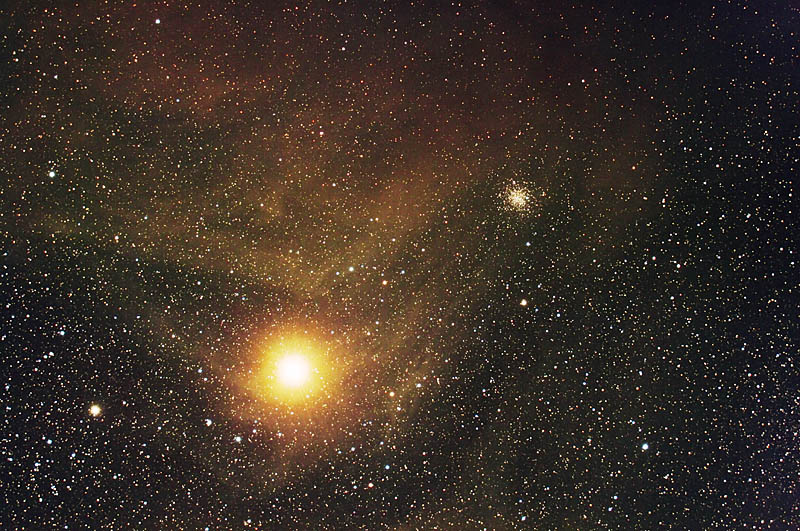
The bright red star Antares, middle, near the prominent star cluster M4, upper right. Photo via Fred Espenak at AstroPixels. Used with permission.

Bright reddish Antares – also known as Alpha Scorpii – is easy to spot on a summer night. It is the brightest star – and distinctly reddish in color – in the fishhook-shaped pattern of stars known as the constellation Scorpius the Scorpion.

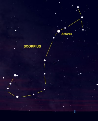
Scorpius is one of the few constellations that looks like its namesake. The bright red star Antares marks the Scorpion’s Heart. Notice also the two stars at the tip of the Scorpion’s Tail. They are known as The Stinger.

How to see Antares. If you look southward in early evening from late spring to early fall, you’re likely to notice the fishhook pattern of Scorpius the Scorpion, with ruby Antares at its heart. If you think you’ve found Antares, aim binoculars in its direction. You should notice its reddish color. And you should see a little star cluster – known as M4 – just to the right of this star. (See images above)

Antares is the 16th brightest star in the sky, and it is located in the southern half of Earth’s sky. So your chance of seeing this star on any given night increases as you go farther southward on Earth’s globe. If you traveled to the Southern Hemisphere – from about 67 degrees south latitude – you’d find that Antares is circumpolar, meaning that it never sets and is visible every night of the year from Earth’s southernmost regions.

We in the Northern Hemisphere know Antares better than several other southern stars that are brighter. That’s because Antares is visible from throughout most of the Northern Hemisphere, short of the Arctic. Well, not quite the Arctic, but anywhere south of 63 degrees north latitude can – at one time or another – see Antares. (Helsinki yes, Fairbanks, no)

The midnight culmination of Antares is on or near June 1. That is when Antares is highest in the sky at midnight (midway between sunset and sunrise). It is highest in the sky at about dawn in early March and at about sunset in early September.

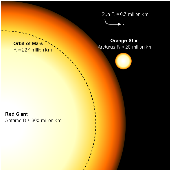
If Antares replaced the sun in our solar system, its circumference would extend beyond the orbit of the fourth planet, Mars. Here, Antares is shown in contrast to another star, Arcturus, and our sun. Image via Wikimedia Commons.

Antares science. Antares is truly an enormous star, with a radius in excess of three astronomical units (AU). One AU is the Earth’s average distance from the sun. If by some bit of magic Antares was suddenly substituted for our sun, the surface of the star would extend well past the orbit of Mars!

Antares is classified as an M1 supergiant star. The M1 designation says that Antares is reddish in color and cooler than many other stars. Its surface temperature of 3500 kelvins (about 5800 degrees F or 3200 C) is in contrast to about 10,000 degrees F (5500 C) for our sun.

Even though Antares’ surface temperature is relatively low, Antares’ tremendous surface area – the surface from which light can escape – makes this star very bright. In fact, Antares approaches 11,000 times the brilliance of our puny sun, a G2 star.

But that is just in visible light. When all wavelengths of electromagnetic radiation are considered, Antares pumps out more than 60,000 times the energy of our sun!

Red Antares is similar to but somewhat larger than another famous red star, Betelgeuse in the constellation Orion. Yet Betelgeuse appears slightly brighter than Antares in our sky. Hipparcos satellite data places Antares at about 604 light-years away, in contrast to Betelgeuse’s distance of 428 light-years, explaining why the larger star appears fainter from Earth.

Like all M-type giants and supergiants, Antares is close to the end of its lifetime. Someday soon (astronomically speaking), it will effectively run out of fuel and collapse. The resulting infall of its enormous mass – some 15-18 times the mass of our sun – will cause an immense supernova explosion, ultimately leaving a tiny neutron star or possibly a black hole. This explosion, which could be tomorrow or millions of years from now, will be spectacular as seen from Earth, but we are far enough away that there likely is no danger to our planet.

Scorpius, via Constellation of Words.

Antares in history and myth. Both the Arabic and Latin names for the star Antares mean “heart of the Scorpion.” If you see this constellation in the sky, you’ll find that Antares does indeed seem to reside at the Scorpion’s heart.

Antares is Greek for “like Mars” or “rivaling Mars.” Antares is sometimes said to be the “anti-Mars.” All of this rivalry (or equivalency … for what is rivalry, after all?) stems from the colors of Mars and Antares. Both are red in color, and, for a few months every couple of years Mars is much brighter than Antares. Most of the time, though, Mars is near the same brightness or much fainter than Antares. Every couple of years, Mars passes near Antares, which was perhaps seen as taunting the star, as Mars moves rapidly through the heavens and Antares, like all stars, seems fixed to the starry firmament.

As is typical, more mythology attends the full constellation of Scorpius than the star Antares. Perhaps the most well known story of Scorpius is that the Earth goddess, Gaia, sent him to sting arrogant Orion, who had claimed his intent to kill all animals on the planet. Scorpius killed Orion, and both were placed in the sky, although in opposite sides of the heavens, positioned as if to show the Scorpion chasing the Mighty Hunter.

Interestingly, Betelgeuse in the constellation Orion is similar in appearance to Antares, although brighter. Betelgeuse is not as associated with Mars as is Antares. Although the planet passes in the vicinity of Betelgeuse every couple of years, it never gets as close as it does to Antares.

In Polynesia, Scorpius is often seen as a fishhook, with some stories describing it as the magic fishhook used by the demigod Maui to pull up land from the ocean floor that became the Hawaiian islands. According to the University of Hawaii’s Institute for Astronomy website, the Hawaiian name for Antares, Lehua-kona, seems to have little to do with the constellation. It means “southern lehua blossom.”

Antares’ position is RA:16h 29m 24s, dec: -26° 25′ 55″.

The red star Antares, lower left, near the prominent star cluster M4, right. Image via Dick Locke.

Bottom line: How to find the star Antares in your night sky.

from EarthSky https://ift.tt/2LhMFTM

The bright red star Antares, middle, near the prominent star cluster M4, upper right. Photo via Fred Espenak at AstroPixels. Used with permission.

Bright reddish Antares – also known as Alpha Scorpii – is easy to spot on a summer night. It is the brightest star – and distinctly reddish in color – in the fishhook-shaped pattern of stars known as the constellation Scorpius the Scorpion.

Scorpius is one of the few constellations that looks like its namesake. The bright red star Antares marks the Scorpion’s Heart. Notice also the two stars at the tip of the Scorpion’s Tail. They are known as The Stinger.

How to see Antares. If you look southward in early evening from late spring to early fall, you’re likely to notice the fishhook pattern of Scorpius the Scorpion, with ruby Antares at its heart. If you think you’ve found Antares, aim binoculars in its direction. You should notice its reddish color. And you should see a little star cluster – known as M4 – just to the right of this star. (See images above)

Antares is the 16th brightest star in the sky, and it is located in the southern half of Earth’s sky. So your chance of seeing this star on any given night increases as you go farther southward on Earth’s globe. If you traveled to the Southern Hemisphere – from about 67 degrees south latitude – you’d find that Antares is circumpolar, meaning that it never sets and is visible every night of the year from Earth’s southernmost regions.

We in the Northern Hemisphere know Antares better than several other southern stars that are brighter. That’s because Antares is visible from throughout most of the Northern Hemisphere, short of the Arctic. Well, not quite the Arctic, but anywhere south of 63 degrees north latitude can – at one time or another – see Antares. (Helsinki yes, Fairbanks, no)

The midnight culmination of Antares is on or near June 1. That is when Antares is highest in the sky at midnight (midway between sunset and sunrise). It is highest in the sky at about dawn in early March and at about sunset in early September.

If Antares replaced the sun in our solar system, its circumference would extend beyond the orbit of the fourth planet, Mars. Here, Antares is shown in contrast to another star, Arcturus, and our sun. Image via Wikimedia Commons.

Antares science. Antares is truly an enormous star, with a radius in excess of three astronomical units (AU). One AU is the Earth’s average distance from the sun. If by some bit of magic Antares was suddenly substituted for our sun, the surface of the star would extend well past the orbit of Mars!

Antares is classified as an M1 supergiant star. The M1 designation says that Antares is reddish in color and cooler than many other stars. Its surface temperature of 3500 kelvins (about 5800 degrees F or 3200 C) is in contrast to about 10,000 degrees F (5500 C) for our sun.

Even though Antares’ surface temperature is relatively low, Antares’ tremendous surface area – the surface from which light can escape – makes this star very bright. In fact, Antares approaches 11,000 times the brilliance of our puny sun, a G2 star.

But that is just in visible light. When all wavelengths of electromagnetic radiation are considered, Antares pumps out more than 60,000 times the energy of our sun!

Red Antares is similar to but somewhat larger than another famous red star, Betelgeuse in the constellation Orion. Yet Betelgeuse appears slightly brighter than Antares in our sky. Hipparcos satellite data places Antares at about 604 light-years away, in contrast to Betelgeuse’s distance of 428 light-years, explaining why the larger star appears fainter from Earth.

Like all M-type giants and supergiants, Antares is close to the end of its lifetime. Someday soon (astronomically speaking), it will effectively run out of fuel and collapse. The resulting infall of its enormous mass – some 15-18 times the mass of our sun – will cause an immense supernova explosion, ultimately leaving a tiny neutron star or possibly a black hole. This explosion, which could be tomorrow or millions of years from now, will be spectacular as seen from Earth, but we are far enough away that there likely is no danger to our planet.

Scorpius, via Constellation of Words.

Antares in history and myth. Both the Arabic and Latin names for the star Antares mean “heart of the Scorpion.” If you see this constellation in the sky, you’ll find that Antares does indeed seem to reside at the Scorpion’s heart.

Antares is Greek for “like Mars” or “rivaling Mars.” Antares is sometimes said to be the “anti-Mars.” All of this rivalry (or equivalency … for what is rivalry, after all?) stems from the colors of Mars and Antares. Both are red in color, and, for a few months every couple of years Mars is much brighter than Antares. Most of the time, though, Mars is near the same brightness or much fainter than Antares. Every couple of years, Mars passes near Antares, which was perhaps seen as taunting the star, as Mars moves rapidly through the heavens and Antares, like all stars, seems fixed to the starry firmament.

As is typical, more mythology attends the full constellation of Scorpius than the star Antares. Perhaps the most well known story of Scorpius is that the Earth goddess, Gaia, sent him to sting arrogant Orion, who had claimed his intent to kill all animals on the planet. Scorpius killed Orion, and both were placed in the sky, although in opposite sides of the heavens, positioned as if to show the Scorpion chasing the Mighty Hunter.

Interestingly, Betelgeuse in the constellation Orion is similar in appearance to Antares, although brighter. Betelgeuse is not as associated with Mars as is Antares. Although the planet passes in the vicinity of Betelgeuse every couple of years, it never gets as close as it does to Antares.

In Polynesia, Scorpius is often seen as a fishhook, with some stories describing it as the magic fishhook used by the demigod Maui to pull up land from the ocean floor that became the Hawaiian islands. According to the University of Hawaii’s Institute for Astronomy website, the Hawaiian name for Antares, Lehua-kona, seems to have little to do with the constellation. It means “southern lehua blossom.”

Antares’ position is RA:16h 29m 24s, dec: -26° 25′ 55″.

The red star Antares, lower left, near the prominent star cluster M4, right. Image via Dick Locke.

Bottom line: How to find the star Antares in your night sky.

from EarthSky https://ift.tt/2LhMFTM

Astronomers spot asteroid with shortest year known

The orbit of asteroid 2019 LF6 (white) falls entirely within the orbit of Earth (blue). Image via NASA/JPL-Caltech.

On July 8, 2019, Caltech astronomers announced their discovery of an unusual asteroid with the shortest year known for any asteroid. The rocky body, dubbed 2019 LF6, is about half a mile (1 km) in size and circles the sun roughly every 151 days.

2019 LF6 is one of only 20 known Atira asteroids, which are objects whose orbits fall entirely within Earth’s path around the sun. That is, their orbit has an aphelion (farthest point from the sun) smaller than Earth’s perihelion (nearest point to the sun). In its orbit, 2019 LF6 swings out beyond Venus and, at times, comes closer to the sun than Mercury, which circles the sun every 88 days.

Quanzhi Ye, a postdoctoral scholar at Caltech, discovered 2019 LF6. He said in a statement:

You don’t find kilometer-size asteroids very often these days. Thirty years ago, people started organizing methodical asteroid searches, finding larger objects first, but now that most of them have been found, the bigger ones are rare birds. LF6 is very unusual both in orbit and in size – its unique orbit explains why such a large asteroid eluded several decades of careful searches.

Asteroid 2019 LF6 is seen here traveling across the sky in images captured on June 10, 2019. The movie has been sped up: the actual time elapsed is 13 minutes. Image via ZTF/Caltech Optical Observatories.

2019 LF6 was discovered via the Zwicky Transient Facility, or ZTF, a state-of-the-art camera at California’s Palomar Observatory that scans the skies every night for transient objects, such as exploding and flashing stars and moving asteroids. Because ZTF scans the sky so rapidly, it is well-suited for finding Atira asteroids, which have short observing windows. Ye said:

We only have about 20 to 30 minutes before sunrise or after sunset to find these asteroids.

The ZTF team has discovered one other Atira asteroid so far, named 2019 AQ3. Before the astronomers spotted 2019 LF6, 2019 AQ3 had the shortest known year of any asteroid, orbiting the sun roughly every 165 days. Tom Prince is a physics professor at Caltech and a senior research scientist at JPL. Prince said:

Both of the large Atira asteroids that were found by ZTF orbit well outside the plane of the solar system. This suggests that sometime in the past they were flung out of the plane of the solar system because they came too close to Venus or Mercury.

Bottom line: Asteroid 2019 LF6 orbits the sun roughly every 151 days, the shortest year yet known for an asteroid.

Via Caltech

from EarthSky https://ift.tt/2JE5tcO

The orbit of asteroid 2019 LF6 (white) falls entirely within the orbit of Earth (blue). Image via NASA/JPL-Caltech.

On July 8, 2019, Caltech astronomers announced their discovery of an unusual asteroid with the shortest year known for any asteroid. The rocky body, dubbed 2019 LF6, is about half a mile (1 km) in size and circles the sun roughly every 151 days.

2019 LF6 is one of only 20 known Atira asteroids, which are objects whose orbits fall entirely within Earth’s path around the sun. That is, their orbit has an aphelion (farthest point from the sun) smaller than Earth’s perihelion (nearest point to the sun). In its orbit, 2019 LF6 swings out beyond Venus and, at times, comes closer to the sun than Mercury, which circles the sun every 88 days.

Quanzhi Ye, a postdoctoral scholar at Caltech, discovered 2019 LF6. He said in a statement:

You don’t find kilometer-size asteroids very often these days. Thirty years ago, people started organizing methodical asteroid searches, finding larger objects first, but now that most of them have been found, the bigger ones are rare birds. LF6 is very unusual both in orbit and in size – its unique orbit explains why such a large asteroid eluded several decades of careful searches.

Asteroid 2019 LF6 is seen here traveling across the sky in images captured on June 10, 2019. The movie has been sped up: the actual time elapsed is 13 minutes. Image via ZTF/Caltech Optical Observatories.

2019 LF6 was discovered via the Zwicky Transient Facility, or ZTF, a state-of-the-art camera at California’s Palomar Observatory that scans the skies every night for transient objects, such as exploding and flashing stars and moving asteroids. Because ZTF scans the sky so rapidly, it is well-suited for finding Atira asteroids, which have short observing windows. Ye said:

We only have about 20 to 30 minutes before sunrise or after sunset to find these asteroids.

The ZTF team has discovered one other Atira asteroid so far, named 2019 AQ3. Before the astronomers spotted 2019 LF6, 2019 AQ3 had the shortest known year of any asteroid, orbiting the sun roughly every 165 days. Tom Prince is a physics professor at Caltech and a senior research scientist at JPL. Prince said:

Both of the large Atira asteroids that were found by ZTF orbit well outside the plane of the solar system. This suggests that sometime in the past they were flung out of the plane of the solar system because they came too close to Venus or Mercury.

Bottom line: Asteroid 2019 LF6 orbits the sun roughly every 151 days, the shortest year yet known for an asteroid.

Via Caltech

from EarthSky https://ift.tt/2JE5tcO

How to see Jupiter’s moons

Composite image of Jupiter and its 4 Galilean moons. From top to bottom the moons are Io, Europa, Ganymede, Callisto. The Galileo spacecraft obtained the images to make this composite in 1996. Image via NASA PhotoJournal.

If you have binoculars or a telescope, it’s fairly easy whenever Jupiter is visible to see the giant planet’s four largest moons. They look like pinpricks of light – like tiny “stars” – all on or near the same plane crossing the planet. They’re often called the Galilean moons to honor Galileo, who discovered them in 1610.

In their order from Jupiter, these moons are Io, Europa, Ganymede and Callisto.

Jupiter and 3 of its 4 Galilean satellites, as they’d appear in a small telescope. Illustration via SkyandTelescope.com.

Writing at SkyandTelescope.com this year, Bob King said:

Etched in my brain cells is an image of a sharp, gleaming disk striped with two dark belts and accompanied by four star-like moons through my 2.4-inch refractor in the winter of 1966. A 6-inch reflector will make you privy to nearly all of the planet’s secrets …

When magnified at 150× or higher [the four Galilean moons] lose their star-like appearance and show disks that range in size from 1.0″ to 1.7″ (current opposition). Europa’s the smallest and Ganymede largest.

Ganymede also casts the largest shadow on the planet’s cloud tops when it transits in front of Jupiter. Shadow transits are visible at least once a week with ‘double transits’ – two moons casting shadows simultaneously – occurring once or twice a month. Ganymede’s shadow looks like a bullet hole, while little Europa’s more resembles a pinprick. Moons also fade away and then reappear over several minutes when they enter and exit Jupiter’s shadow during eclipse. Or a moon may be occulted by the Jovian disk and hover at the planet’s edge like a pearl before fading from sight.

You’ll find a complete list of all eclipses, transits, and occultations for 2019 by downloading Sky & Telescope’s Phenomena of Jupiter’s Moons pdf. You can also gets daily predictions for the moons and a diagram showing their relative positions by consulting the online Jupiter’s Moons Observing Tool.

Read more: We go between the sun and Jupiter

View at EarthSky Community Photos. | Beautiful shot of Earth’s moon – plus Jupiter and its 4 largest moons – on May 20, 2019, via Asthadi Setyawan in Malang, East Java, Indonesia. Thank you, Asthadi!

The Galilean moons orbit Jupiter around its equator. We do see their orbits almost exactly edge-on, but, as with so much in astronomy, there’s a cycle for viewing the edge-on-ness of Jupiter’s moons. This particular cycle is six years long. That is, every six years, we view Jupiter’s equator – and the moons orbiting above its equator – most edge-on.

And that’s why, in 2015, we were able to view a number of mutual events (eclipses and shadow transits) involving Jupiter’s moons, through telescopes.

Starting in late 2016, Jupiter’s axis began tilting enough toward the sun and Earth so that the outermost of the four moons, Callisto, had not been passing in front of Jupiter or behind Jupiter, as seen from our vantage point. This will continue for a period of about three years, during which time Callisto is perpetually visible to those with telescopes, alternately swinging above and below Jupiter as seen from Earth.

The next eclipse series of Callisto, whereby this moon actually passes behind Jupiter, starts on November 9, 2019, and ends on August 22, 2022, to present a total of 61 eclipses. After that, the next eclipse series will occur from May 29, 2025, to June 7, 2028, to feature 67 eclipses.

Click here for a Jupiter’s moons almanac, courtesy of SkyandTelescope.com.

Click here for recommended sky almanacs; they can tell you Jupiter’s rising time in your sky.

Fernando Roquel Torres in Caguas, Puerto Rico, captured Jupiter, its Great Red Spot and all 4 of its largest moons – the Galilean satellites – at Jupiter’s 2017 opposition.

Bottom line: How to see Jupiter’s moons.

from EarthSky https://ift.tt/2LhWrFE

Composite image of Jupiter and its 4 Galilean moons. From top to bottom the moons are Io, Europa, Ganymede, Callisto. The Galileo spacecraft obtained the images to make this composite in 1996. Image via NASA PhotoJournal.

If you have binoculars or a telescope, it’s fairly easy whenever Jupiter is visible to see the giant planet’s four largest moons. They look like pinpricks of light – like tiny “stars” – all on or near the same plane crossing the planet. They’re often called the Galilean moons to honor Galileo, who discovered them in 1610.

In their order from Jupiter, these moons are Io, Europa, Ganymede and Callisto.

Jupiter and 3 of its 4 Galilean satellites, as they’d appear in a small telescope. Illustration via SkyandTelescope.com.

Writing at SkyandTelescope.com this year, Bob King said:

Etched in my brain cells is an image of a sharp, gleaming disk striped with two dark belts and accompanied by four star-like moons through my 2.4-inch refractor in the winter of 1966. A 6-inch reflector will make you privy to nearly all of the planet’s secrets …

When magnified at 150× or higher [the four Galilean moons] lose their star-like appearance and show disks that range in size from 1.0″ to 1.7″ (current opposition). Europa’s the smallest and Ganymede largest.

Ganymede also casts the largest shadow on the planet’s cloud tops when it transits in front of Jupiter. Shadow transits are visible at least once a week with ‘double transits’ – two moons casting shadows simultaneously – occurring once or twice a month. Ganymede’s shadow looks like a bullet hole, while little Europa’s more resembles a pinprick. Moons also fade away and then reappear over several minutes when they enter and exit Jupiter’s shadow during eclipse. Or a moon may be occulted by the Jovian disk and hover at the planet’s edge like a pearl before fading from sight.

You’ll find a complete list of all eclipses, transits, and occultations for 2019 by downloading Sky & Telescope’s Phenomena of Jupiter’s Moons pdf. You can also gets daily predictions for the moons and a diagram showing their relative positions by consulting the online Jupiter’s Moons Observing Tool.

Read more: We go between the sun and Jupiter

View at EarthSky Community Photos. | Beautiful shot of Earth’s moon – plus Jupiter and its 4 largest moons – on May 20, 2019, via Asthadi Setyawan in Malang, East Java, Indonesia. Thank you, Asthadi!

The Galilean moons orbit Jupiter around its equator. We do see their orbits almost exactly edge-on, but, as with so much in astronomy, there’s a cycle for viewing the edge-on-ness of Jupiter’s moons. This particular cycle is six years long. That is, every six years, we view Jupiter’s equator – and the moons orbiting above its equator – most edge-on.

And that’s why, in 2015, we were able to view a number of mutual events (eclipses and shadow transits) involving Jupiter’s moons, through telescopes.

Starting in late 2016, Jupiter’s axis began tilting enough toward the sun and Earth so that the outermost of the four moons, Callisto, had not been passing in front of Jupiter or behind Jupiter, as seen from our vantage point. This will continue for a period of about three years, during which time Callisto is perpetually visible to those with telescopes, alternately swinging above and below Jupiter as seen from Earth.

The next eclipse series of Callisto, whereby this moon actually passes behind Jupiter, starts on November 9, 2019, and ends on August 22, 2022, to present a total of 61 eclipses. After that, the next eclipse series will occur from May 29, 2025, to June 7, 2028, to feature 67 eclipses.

Click here for a Jupiter’s moons almanac, courtesy of SkyandTelescope.com.

Click here for recommended sky almanacs; they can tell you Jupiter’s rising time in your sky.

Fernando Roquel Torres in Caguas, Puerto Rico, captured Jupiter, its Great Red Spot and all 4 of its largest moons – the Galilean satellites – at Jupiter’s 2017 opposition.

Bottom line: How to see Jupiter’s moons.

from EarthSky https://ift.tt/2LhWrFE

Moon to sweep by Jupiter July 12 to 14

On the evenings of July 12, 13 and 14, 2019, watch for the bright waxing gibbous moon to swing by the giant planet Jupiter. Fortunately, the king planet is so bright that this world can easily withstand the lunar glare. After all, Jupiter is the 4th-brightest light in the heavens, after the sun, moon and planet Venus. Venus is a morning object, virtually lost in the sun’s glare now, so there’s no way to mistake Venus for Jupiter in the July evening sky.

Although the moon and Jupiter appear close together on the sky’s dome, these two worlds are nowhere close to one another in space. The moon, our closest celestial neighbor, is around its average distance from Earth (238,955 miles or 384,400 km) right now. Jupiter resides more than 1,700 times the moon’s distance from Earth. At present, Jupiter lies 4.42 astronomical units (AU) from Earth. One AU = one Earth-sun distance = 92,955,817 miles or 149,597,871 km. Jupiter is currently 5.29 AU from the sun.

Click here to learn the moon’s present distance in miles, kilometers and AU.

Click here to know Jupiter’s present distance in AU.

View at EarthSky Community Photos. | If you can learn to identify Jupiter this weekend, you’ll enjoy it even more in dark country sky, after the moon has moved away. Jupiter is the brightest starlike object in the night sky now, as seen in this image captured by Kristopher Schoenleber on July 5, 2019 near Winthrop, Washington. Jupiter is now located in our sky next to the starry band of the Milky Way. Thank you, Kristopher!

After the moon and Jupiter first come out at dusk, the brilliant twosome will continue to move westward across the sky throughout the night. They’ll set beneath the southwest horizon in the wee hours before dawn. The moon and Jupiter (plus the nearby star Antares) all cross the sky for the same reason that the sun travels westward across the sky during the daylight hours, because Earth spins eastward under the sky. The Earth’s spin on its axis – from west-to-east – causes the sun, moon stars and planets to go full circle around our sky each day.

Even though, as Earth spins, the moon goes westward throughout the night, it is also moving eastward in front of the background stars and planets of the zodiac. The moon’s eastward motion in front of the stars is its true motion in orbit around Earth. As darkness falls on July 12, note the moon’s position relative to Jupiter and the star Antares. Then, at nightfall on July 13, note how much more closely the moon couples up with Jupiter. That’s because, as measured by the backdrop stars of the zodiac, the moon in its orbit travels about 1/2 degree (its own angular diameter) eastward per hour. That equals about 13 degrees eastward per day.

Jupiter is big! Its Great Red Spot – which, by the way, has been behaving strangely in recent months – is about the size of Earth. You’d need 11 Earths lined up side by side to equal the diameter of Jupiter. Image via Wikimedia Commons.

The moon appears so much larger than Jupiter in our sky because it’s so much closer to us than Jupiter. If you want to get some idea of the moon’s size relative to Jupiter, look at the king planet through the telescope sometime. Jupiter’s four major moons – Io, Europa, Ganymede and Callisto – are quite easy to view through a low-powered telescope. Two of these moons – Ganymede and Callisto – have diameters about 1 1/2 times that of Earth’s moon, whereas the other two – Io and Europa – are approximately the same size as our moon. Find out the present positions of Jupiter’s four major moons via SkyandTelescope.com.

Read more: How Jupiter’s moons reveal Jupiter’s mass

The Galilean moons, in their order going outward, from Left to right: Io, Europa, Ganymede and Callisto

Bottom line: Use the moon to locate the planet Jupiter on July 12, 13 and 14. After these nights, you’ll recognize Jupiter easily. It’ll be the brightest starlike object to light up the evening sky for months to come.

from EarthSky https://ift.tt/2JEEXQw

On the evenings of July 12, 13 and 14, 2019, watch for the bright waxing gibbous moon to swing by the giant planet Jupiter. Fortunately, the king planet is so bright that this world can easily withstand the lunar glare. After all, Jupiter is the 4th-brightest light in the heavens, after the sun, moon and planet Venus. Venus is a morning object, virtually lost in the sun’s glare now, so there’s no way to mistake Venus for Jupiter in the July evening sky.

Although the moon and Jupiter appear close together on the sky’s dome, these two worlds are nowhere close to one another in space. The moon, our closest celestial neighbor, is around its average distance from Earth (238,955 miles or 384,400 km) right now. Jupiter resides more than 1,700 times the moon’s distance from Earth. At present, Jupiter lies 4.42 astronomical units (AU) from Earth. One AU = one Earth-sun distance = 92,955,817 miles or 149,597,871 km. Jupiter is currently 5.29 AU from the sun.

Click here to learn the moon’s present distance in miles, kilometers and AU.

Click here to know Jupiter’s present distance in AU.

View at EarthSky Community Photos. | If you can learn to identify Jupiter this weekend, you’ll enjoy it even more in dark country sky, after the moon has moved away. Jupiter is the brightest starlike object in the night sky now, as seen in this image captured by Kristopher Schoenleber on July 5, 2019 near Winthrop, Washington. Jupiter is now located in our sky next to the starry band of the Milky Way. Thank you, Kristopher!

After the moon and Jupiter first come out at dusk, the brilliant twosome will continue to move westward across the sky throughout the night. They’ll set beneath the southwest horizon in the wee hours before dawn. The moon and Jupiter (plus the nearby star Antares) all cross the sky for the same reason that the sun travels westward across the sky during the daylight hours, because Earth spins eastward under the sky. The Earth’s spin on its axis – from west-to-east – causes the sun, moon stars and planets to go full circle around our sky each day.

Even though, as Earth spins, the moon goes westward throughout the night, it is also moving eastward in front of the background stars and planets of the zodiac. The moon’s eastward motion in front of the stars is its true motion in orbit around Earth. As darkness falls on July 12, note the moon’s position relative to Jupiter and the star Antares. Then, at nightfall on July 13, note how much more closely the moon couples up with Jupiter. That’s because, as measured by the backdrop stars of the zodiac, the moon in its orbit travels about 1/2 degree (its own angular diameter) eastward per hour. That equals about 13 degrees eastward per day.

Jupiter is big! Its Great Red Spot – which, by the way, has been behaving strangely in recent months – is about the size of Earth. You’d need 11 Earths lined up side by side to equal the diameter of Jupiter. Image via Wikimedia Commons.

The moon appears so much larger than Jupiter in our sky because it’s so much closer to us than Jupiter. If you want to get some idea of the moon’s size relative to Jupiter, look at the king planet through the telescope sometime. Jupiter’s four major moons – Io, Europa, Ganymede and Callisto – are quite easy to view through a low-powered telescope. Two of these moons – Ganymede and Callisto – have diameters about 1 1/2 times that of Earth’s moon, whereas the other two – Io and Europa – are approximately the same size as our moon. Find out the present positions of Jupiter’s four major moons via SkyandTelescope.com.

Read more: How Jupiter’s moons reveal Jupiter’s mass

The Galilean moons, in their order going outward, from Left to right: Io, Europa, Ganymede and Callisto

Bottom line: Use the moon to locate the planet Jupiter on July 12, 13 and 14. After these nights, you’ll recognize Jupiter easily. It’ll be the brightest starlike object to light up the evening sky for months to come.

from EarthSky https://ift.tt/2JEEXQw

Himalayan glaciers melting double fast since 2000

This article is republished with permission from GlacierHub. This post was written by Elza Bouhassira.

The Himalayas have a powerful impact on the lives of the people who live near them: They have cultural and religious sway, they play a role in determining regional weather patterns, and they feed major rivers like the Indus, the Ganges, and the Tsangpo-Brahmaputra that millions rely on for fresh water.

A new study published June 19, 2019, in the journal Science Advances by Ph.D. candidate Joshua Maurer of Columbia University’s Lamont-Doherty Earth Observatory concludes that glaciers in the Himalayas melted twice as quickly from 2000 to 2016 than they did from 1975 to 2000. Maurer said:

This is the clearest picture yet of how fast Himalayan glaciers are melting over this time interval, and why.

Spiti Valley, which means “The Middle Land,” is located in the northern Indian province of Himachal Pradesh in the Himalayas. Image via beagle17/Creative Commons.

Walter Immerzeel, a professor in the University of Utrecht’s department of geosciences, told GlacierHub that

… the novelty lies in the fact that they go back until 1975.

He said that scientists already knew “quite well” what the mass balance rates were for the last twenty years or so, but that looking further back and over a wider area provided interesting new information.

Maurer and his co-authors examined ice loss along a 1,200-mile (2,000-km) long transect of the Himalayas, from western India eastwards to Bhutan. The study area includes 650 of the largest glaciers in the Himalayas and confirms the results of previous studies conducted by researchers who looked at the rate of mass loss in the Himalayas.

The new study makes a major contribution by indicating that regional warming is responsible for the increase in melting. The researchers were able to determine this because mass loss rates were similar across subregions despite variations in other factors like air pollution and precipitation that can also accelerate melting.

Immerzeel agreed with the findings. He said:

It is mostly temperature change driving the mass balances. It can be locally enforced by black carbon or modulated by precipitation changes, but the main driving force is a rise in temperature.

A diagram of a KH-9 Hexagon satellite that was used to create the images used in Maurer’s study. Image via National Reconnaissance Office.

The analysis was conducted using images from declassified KH-9 Hexagon spy satellites which were used by U.S. intelligence agencies during the Cold War. The satellites orbited Earth between 1973 and 1980, taking 29,000 images that were kept as government secrets until relatively recently when they were declassified, creating a cornucopia of data for researchers to comb through.

Maurer and his co-authors used the images to build models showing the size of the glaciers when the images were created. The historical models were then compared to more recent satellite images to determine the changes that occurred over time. Only glaciers for which data were available during both time periods were included in the study.

The new study received widespread media attention. National Geographic, CNN, the New Yorker, and The Guardian, among other major publications, highlighted the study’s conclusion that mass loss in Himalayan glaciers has doubled in the last forty years.

Tobias Bolch, a glaciologist at the University of St Andrews, told GlacierHub the findings should be approached with caution. He said:

The statement about the doubling of the mass loss after 2000 compared to the period 1975-2000 should be formulated with much more care.

[Scientists] need to be very careful presenting results about Himalayan glaciers and should communicate them correctly specifically after the IPCC AR4 error, and the wrong statement about the rapid disappearance of Himalayan glaciers.

Bloch is referring to an error that occurred in 2007, when the IPCC included in its Fourth Assessment Report an inaccurate statement predicting that all Himalayan glaciers would be gone by 2035. He said:

It is a promising data set, but due to its nature there are large data gaps which need to be filled which makes the data uncertain.

He added that there is “clear evidence” that mass loss has accelerated in the Himalayas.

A stretch of the Indus River. Image via arsalank2/Creative Commons.

A recent report by the International Centre for Integrated Mountain Development, a regional intergovernmental organization in Nepal working on sustainable development in mountains, predicts that the Himalayas could lose 64 percent of their ice by the year 2100.

Maurer’s study examines only past melting from 1975 to 2016. ICIMOD’s study provides additional dimensions to Maurer’s results.

The large amount of melting that may occur in the coming decades would result in greater quantities of meltwater entering rivers. The Indus River, which millions rely on for drinking water and agriculture, receives about 40 percent of its flow from glacial melt. An increase in meltwater could augment the risk of flooding of the Indus and other rivers in the region.

Similarly, there may be a greater number of glacial outburst floods. Outburst floods occur when the moraine, or rock wall, which acts as a dam, collapses. A collapse can take place for various reasons including if a great deal of water accumulates in a lake from a phenomenon like an increase in glacial melting. Depending on the size of the lake and downstream populations, among other factors, these floods have the potential to cause substantial damage. The largest of these floods have killed thousands of people, swept away homes, and even registered on seismometers in Nepal.

Reflections in a glacial lake in Norway. Image via Peter Nijenhuis/Flickr.

Once glaciers have lost substantial amounts of mass and no longer have large quantities of water to release, the reverse will begin to cause problems: Rivers dependent on Himalayan glacial melt will diminish and drought may become more common downstream. This will negatively affect farming and development in the Himalayan region.

In both the short and long term, according Maurer and his colleagues, glacier melt in the Himalayas will have significant impacts on the livelihoods of those dependent on its towering peaks.

Bottom line: According to a new study, Himalayan glaciers melted twice as fast from 2000 to 2016 as they did from 1975 to 2000.

from EarthSky https://ift.tt/2SfulLS

This article is republished with permission from GlacierHub. This post was written by Elza Bouhassira.

The Himalayas have a powerful impact on the lives of the people who live near them: They have cultural and religious sway, they play a role in determining regional weather patterns, and they feed major rivers like the Indus, the Ganges, and the Tsangpo-Brahmaputra that millions rely on for fresh water.

A new study published June 19, 2019, in the journal Science Advances by Ph.D. candidate Joshua Maurer of Columbia University’s Lamont-Doherty Earth Observatory concludes that glaciers in the Himalayas melted twice as quickly from 2000 to 2016 than they did from 1975 to 2000. Maurer said:

This is the clearest picture yet of how fast Himalayan glaciers are melting over this time interval, and why.

Spiti Valley, which means “The Middle Land,” is located in the northern Indian province of Himachal Pradesh in the Himalayas. Image via beagle17/Creative Commons.

Walter Immerzeel, a professor in the University of Utrecht’s department of geosciences, told GlacierHub that

… the novelty lies in the fact that they go back until 1975.

He said that scientists already knew “quite well” what the mass balance rates were for the last twenty years or so, but that looking further back and over a wider area provided interesting new information.

Maurer and his co-authors examined ice loss along a 1,200-mile (2,000-km) long transect of the Himalayas, from western India eastwards to Bhutan. The study area includes 650 of the largest glaciers in the Himalayas and confirms the results of previous studies conducted by researchers who looked at the rate of mass loss in the Himalayas.

The new study makes a major contribution by indicating that regional warming is responsible for the increase in melting. The researchers were able to determine this because mass loss rates were similar across subregions despite variations in other factors like air pollution and precipitation that can also accelerate melting.

Immerzeel agreed with the findings. He said:

It is mostly temperature change driving the mass balances. It can be locally enforced by black carbon or modulated by precipitation changes, but the main driving force is a rise in temperature.

A diagram of a KH-9 Hexagon satellite that was used to create the images used in Maurer’s study. Image via National Reconnaissance Office.

The analysis was conducted using images from declassified KH-9 Hexagon spy satellites which were used by U.S. intelligence agencies during the Cold War. The satellites orbited Earth between 1973 and 1980, taking 29,000 images that were kept as government secrets until relatively recently when they were declassified, creating a cornucopia of data for researchers to comb through.

Maurer and his co-authors used the images to build models showing the size of the glaciers when the images were created. The historical models were then compared to more recent satellite images to determine the changes that occurred over time. Only glaciers for which data were available during both time periods were included in the study.

The new study received widespread media attention. National Geographic, CNN, the New Yorker, and The Guardian, among other major publications, highlighted the study’s conclusion that mass loss in Himalayan glaciers has doubled in the last forty years.

Tobias Bolch, a glaciologist at the University of St Andrews, told GlacierHub the findings should be approached with caution. He said:

The statement about the doubling of the mass loss after 2000 compared to the period 1975-2000 should be formulated with much more care.

[Scientists] need to be very careful presenting results about Himalayan glaciers and should communicate them correctly specifically after the IPCC AR4 error, and the wrong statement about the rapid disappearance of Himalayan glaciers.

Bloch is referring to an error that occurred in 2007, when the IPCC included in its Fourth Assessment Report an inaccurate statement predicting that all Himalayan glaciers would be gone by 2035. He said:

It is a promising data set, but due to its nature there are large data gaps which need to be filled which makes the data uncertain.

He added that there is “clear evidence” that mass loss has accelerated in the Himalayas.

A stretch of the Indus River. Image via arsalank2/Creative Commons.

A recent report by the International Centre for Integrated Mountain Development, a regional intergovernmental organization in Nepal working on sustainable development in mountains, predicts that the Himalayas could lose 64 percent of their ice by the year 2100.

Maurer’s study examines only past melting from 1975 to 2016. ICIMOD’s study provides additional dimensions to Maurer’s results.

The large amount of melting that may occur in the coming decades would result in greater quantities of meltwater entering rivers. The Indus River, which millions rely on for drinking water and agriculture, receives about 40 percent of its flow from glacial melt. An increase in meltwater could augment the risk of flooding of the Indus and other rivers in the region.

Similarly, there may be a greater number of glacial outburst floods. Outburst floods occur when the moraine, or rock wall, which acts as a dam, collapses. A collapse can take place for various reasons including if a great deal of water accumulates in a lake from a phenomenon like an increase in glacial melting. Depending on the size of the lake and downstream populations, among other factors, these floods have the potential to cause substantial damage. The largest of these floods have killed thousands of people, swept away homes, and even registered on seismometers in Nepal.

Reflections in a glacial lake in Norway. Image via Peter Nijenhuis/Flickr.

Once glaciers have lost substantial amounts of mass and no longer have large quantities of water to release, the reverse will begin to cause problems: Rivers dependent on Himalayan glacial melt will diminish and drought may become more common downstream. This will negatively affect farming and development in the Himalayan region.

In both the short and long term, according Maurer and his colleagues, glacier melt in the Himalayas will have significant impacts on the livelihoods of those dependent on its towering peaks.

Bottom line: According to a new study, Himalayan glaciers melted twice as fast from 2000 to 2016 as they did from 1975 to 2000.

from EarthSky https://ift.tt/2SfulLS

Moon’s near side is its dark side

Tonight, while the moon is a few days shy of meeting up with the king planet Jupiter, let’s see if we can make out the dark areas on tonight’s waxing gibbous moon. These smooth, low-lying lunar plains are called maria, the plural for the word mare, the Latin word for sea. You should be able to see the darkened portions on the moon with the eye alone. The dark maria on the moon’s near side – the solidified remnants of ancient lunar seas of molten magma – make the near side of the moon reflect less light than the far side, which has fewer maria.

So, in terms of albedo or reflectivity, the moon’s dark side is its near side.

Image of the July 11th waxing gibbous moon via the US Naval Observatory

If you’d like to scrutinize the maria more closely, use binoculars or the telescope. Remember, the view will be better around the time of sunset or early dusk – before the dark of night accentuates the moon’s harsh glare.

In times past, astronomers really thought the dark areas contrasting with the light-colored, heavily-crated highlands were lunar seas. In some ways they were correct, except that these were seas of molten magma instead of water. Now solidified, this molten rock came from volcanic eruptions that flooded the lunar lowlands. However, volcanic activity – at least from basaltic volcanoes – is now a thing of the moon’s past.

For the most part, lunar maria are found on the near side of the moon. In this respect, that makes the near side – not the far side – the dark side of the moon.

Near side of the moon. Click here for a larger image

Far side of the moon via Wikimedia Commons.

Maria cover about 30% of the near side but only 2% of the far side. The reason for this is not well understood, but it has been suggested that the crust on the moon’s far side is thicker, making it more difficult for magma to reach the surface.

The lighter-colored highland regions of the moon are composed of anorthosite, a certain kind of igneous rock. On Earth, anorthosite is uncommon, except for in the Adirondack Mountains and the Canadian Shield. For this reason, people in this part of the world like to fancy that the moon originated from their home turf.

The prevailing theory states that the moon was formed when a Mars-sized object crashed into the Earth, creating a ring of debris that eventually condensed into the moon. I suppose time will tell whether this explanation for the moon’s origin is true or false.

Read more: Far side of moon mystery solved

Bottom line: Strange as it may seem, the moon’s dark side is its near side. By that we mean the near side of the moon reflects less light – due to a collection of dark, low-lying lunar plains that are the solidified remnants of ancient seas of molten magma.

Help support EarthSky! Visit the EarthSky store for to see the great selection of educational tools and team gear we have to offer.

from EarthSky https://ift.tt/2JAoQTW

Tonight, while the moon is a few days shy of meeting up with the king planet Jupiter, let’s see if we can make out the dark areas on tonight’s waxing gibbous moon. These smooth, low-lying lunar plains are called maria, the plural for the word mare, the Latin word for sea. You should be able to see the darkened portions on the moon with the eye alone. The dark maria on the moon’s near side – the solidified remnants of ancient lunar seas of molten magma – make the near side of the moon reflect less light than the far side, which has fewer maria.

So, in terms of albedo or reflectivity, the moon’s dark side is its near side.

Image of the July 11th waxing gibbous moon via the US Naval Observatory

If you’d like to scrutinize the maria more closely, use binoculars or the telescope. Remember, the view will be better around the time of sunset or early dusk – before the dark of night accentuates the moon’s harsh glare.

In times past, astronomers really thought the dark areas contrasting with the light-colored, heavily-crated highlands were lunar seas. In some ways they were correct, except that these were seas of molten magma instead of water. Now solidified, this molten rock came from volcanic eruptions that flooded the lunar lowlands. However, volcanic activity – at least from basaltic volcanoes – is now a thing of the moon’s past.

For the most part, lunar maria are found on the near side of the moon. In this respect, that makes the near side – not the far side – the dark side of the moon.

Near side of the moon. Click here for a larger image

Far side of the moon via Wikimedia Commons.

Maria cover about 30% of the near side but only 2% of the far side. The reason for this is not well understood, but it has been suggested that the crust on the moon’s far side is thicker, making it more difficult for magma to reach the surface.

The lighter-colored highland regions of the moon are composed of anorthosite, a certain kind of igneous rock. On Earth, anorthosite is uncommon, except for in the Adirondack Mountains and the Canadian Shield. For this reason, people in this part of the world like to fancy that the moon originated from their home turf.

The prevailing theory states that the moon was formed when a Mars-sized object crashed into the Earth, creating a ring of debris that eventually condensed into the moon. I suppose time will tell whether this explanation for the moon’s origin is true or false.

Read more: Far side of moon mystery solved

Bottom line: Strange as it may seem, the moon’s dark side is its near side. By that we mean the near side of the moon reflects less light – due to a collection of dark, low-lying lunar plains that are the solidified remnants of ancient seas of molten magma.

Help support EarthSky! Visit the EarthSky store for to see the great selection of educational tools and team gear we have to offer.

from EarthSky https://ift.tt/2JAoQTW

Dust storms swirl at Mars’ north pole

In late May 2019, a spiral-shaped dust storm at the north polar ice cap of Mars was observed by several instruments onboard Mars Express. A Mars Express camera captured this image on May 26. The dust storm’s brown color contrasts with the white ice of the north polar ice cap below. The image covers area of about 1,200 x 3,000 miles (2,000 x 5,000 km). See a larger image. Image via ESA.

The European Space Agency’s (ESA) Mars Express spacecraft has been monitoring dust storms brewing at Mars’ north pole over the last month, and watching as the storms disperse towards the equator. The spacecraft observed at least eight different storms at the edge of the ice cap between May 22 and June 10, 2019, which formed and dissipated very quickly, between one and three days.

It’s currently spring in the northern hemisphere of Mars, and water-ice clouds and small dust-lifting events are frequently observed along the edge of the seasonally retreating ice cap. Local and regional storms lasting for a few days or weeks and confined to a small area are common on Mars, but at their most severe can engulf the entire planet, as experienced last year in a global storm that circled the planet for many months.

Mars dust storm in motion. This animated sequence was compiled from images of a different storm captured by the VMC over a period of 70 minutes on 29 May 29, 2019. This particular storm started on May 28 and continued to around June 1, moving towards the equator during that time. Image via ESA/GCP/UPV/EHU Bilbao.

This montage of images shows 3 different storms developing on May 22, 2019, on May 26, and between June 6 and 10. In the latter case, the cameras watched the storm evolve for several days as it moved in an equator-ward direction. At the same time, wispy patches of light-coloured clouds can be seen at the outer margin of the polar cap and also several thousand kilometres away, close to the volcanoes Elysium Mons and Olympus Mons. Image via ESA/DLR/FU Berlin

Both Mars Express and NASA’s Mars Reconnaissance Orbiter observed that when the dust storms reached the large volcanoes Elysium Mons and Olympus Mons, orographic clouds – water ice clouds driven by the influence of the volcano’s leeward slope on the air flow – that had been developing, started to evaporate as a result of the air mass being heated by the influx of dust.

These regional dust storms only last a few days. The planet’s circulation moves the elevated dust spreads it out into a thin haze in the lower atmosphere. Some traces of dust and clouds remained in the volcanic province into mid-June.

A dust storm underway at the edge of the north polar ice cap of Mars. The image was taken by the Mars Express Visual Monitoring Camera on 29 May 2019. Image via ESA/GCP/UPV/EHU Bilbao

Look out for dust storms in the daily images provided by the ESA’s Mars webcam, on Flickr and Twitter.

Bottom line: Images of dust storms at the Mars north pole, take by ESA’s Mars Express.

Via ESA

from EarthSky https://ift.tt/2Ju5RvH

In late May 2019, a spiral-shaped dust storm at the north polar ice cap of Mars was observed by several instruments onboard Mars Express. A Mars Express camera captured this image on May 26. The dust storm’s brown color contrasts with the white ice of the north polar ice cap below. The image covers area of about 1,200 x 3,000 miles (2,000 x 5,000 km). See a larger image. Image via ESA.

The European Space Agency’s (ESA) Mars Express spacecraft has been monitoring dust storms brewing at Mars’ north pole over the last month, and watching as the storms disperse towards the equator. The spacecraft observed at least eight different storms at the edge of the ice cap between May 22 and June 10, 2019, which formed and dissipated very quickly, between one and three days.

It’s currently spring in the northern hemisphere of Mars, and water-ice clouds and small dust-lifting events are frequently observed along the edge of the seasonally retreating ice cap. Local and regional storms lasting for a few days or weeks and confined to a small area are common on Mars, but at their most severe can engulf the entire planet, as experienced last year in a global storm that circled the planet for many months.

Mars dust storm in motion. This animated sequence was compiled from images of a different storm captured by the VMC over a period of 70 minutes on 29 May 29, 2019. This particular storm started on May 28 and continued to around June 1, moving towards the equator during that time. Image via ESA/GCP/UPV/EHU Bilbao.

This montage of images shows 3 different storms developing on May 22, 2019, on May 26, and between June 6 and 10. In the latter case, the cameras watched the storm evolve for several days as it moved in an equator-ward direction. At the same time, wispy patches of light-coloured clouds can be seen at the outer margin of the polar cap and also several thousand kilometres away, close to the volcanoes Elysium Mons and Olympus Mons. Image via ESA/DLR/FU Berlin

Both Mars Express and NASA’s Mars Reconnaissance Orbiter observed that when the dust storms reached the large volcanoes Elysium Mons and Olympus Mons, orographic clouds – water ice clouds driven by the influence of the volcano’s leeward slope on the air flow – that had been developing, started to evaporate as a result of the air mass being heated by the influx of dust.

These regional dust storms only last a few days. The planet’s circulation moves the elevated dust spreads it out into a thin haze in the lower atmosphere. Some traces of dust and clouds remained in the volcanic province into mid-June.

A dust storm underway at the edge of the north polar ice cap of Mars. The image was taken by the Mars Express Visual Monitoring Camera on 29 May 2019. Image via ESA/GCP/UPV/EHU Bilbao

Look out for dust storms in the daily images provided by the ESA’s Mars webcam, on Flickr and Twitter.

Bottom line: Images of dust storms at the Mars north pole, take by ESA’s Mars Express.

Via ESA

from EarthSky https://ift.tt/2Ju5RvH

Today in science: 1st Telstar launch

1962 artist’s concept of Telstar satellite orbiting in space. Image via AT&T/SuperStock/Corbis/NASA.

July 10, 1962. This date marks the launch of Telstar 1, the first communications satellite capable of relaying television signals from Europe to North America, by a Delta rocket.

Telstar – a 171-pound, 34.5-inch sphere loaded with transistors and covered with solar panels – relayed its first signal just hours after its launch from Cape Canaveral, Florida.

A Thor/Delta 316 launches with the Telstar 1 satellite from Cape Canaveral on July 10, 1962. Image via NASA.

The first transmitted images showed an American flag outside a receiving station in Andover, Maine. Later, Telstar sent live television images as well as telephone calls, faxes and other data.

An early transatlantic transmission over Telstar. Image via Daily Mail.

President John F. Kennedy said after Telstar’s launch:

This (is an) outstanding symbol of America’s space achievements.

And so it was. Telstar 1 led to the advent of 24-hour, live news programming from anywhere in the world, an innovation that began to hit its stride during the Vietnam War in the late 1960s and early 1970s.

Meanwhile, anyone old enough to listen to radio in 1962 remembers the hit song “Telstar” an instrumental performed by The Tornados. It reached No. 1 on the U.S. Billboard Hot 100 in December 1962. You can hear a version of Telstar by The Ventures in the video below:

Bottom line: Telstar 1, the first communications satellite capable of relaying television signals from Europe to North America, launched on this date … and helped change the world.

from EarthSky https://ift.tt/2XFbNWr

1962 artist’s concept of Telstar satellite orbiting in space. Image via AT&T/SuperStock/Corbis/NASA.

July 10, 1962. This date marks the launch of Telstar 1, the first communications satellite capable of relaying television signals from Europe to North America, by a Delta rocket.

Telstar – a 171-pound, 34.5-inch sphere loaded with transistors and covered with solar panels – relayed its first signal just hours after its launch from Cape Canaveral, Florida.

A Thor/Delta 316 launches with the Telstar 1 satellite from Cape Canaveral on July 10, 1962. Image via NASA.

The first transmitted images showed an American flag outside a receiving station in Andover, Maine. Later, Telstar sent live television images as well as telephone calls, faxes and other data.

An early transatlantic transmission over Telstar. Image via Daily Mail.

President John F. Kennedy said after Telstar’s launch:

This (is an) outstanding symbol of America’s space achievements.

And so it was. Telstar 1 led to the advent of 24-hour, live news programming from anywhere in the world, an innovation that began to hit its stride during the Vietnam War in the late 1960s and early 1970s.

Meanwhile, anyone old enough to listen to radio in 1962 remembers the hit song “Telstar” an instrumental performed by The Tornados. It reached No. 1 on the U.S. Billboard Hot 100 in December 1962. You can hear a version of Telstar by The Ventures in the video below:

Bottom line: Telstar 1, the first communications satellite capable of relaying television signals from Europe to North America, launched on this date … and helped change the world.

from EarthSky https://ift.tt/2XFbNWr

Rare lava lake seen from space

Mount Michael in the South Sandwich Islands, with its lava lake at the top of the volcano, as seen from space. Image via the Copernicus Sentinel-2 mission/ESA.

The European Space Agency (ESA) released this image on July 4, 2019 and said:

Mount Michael is an active stratovolcano on the remote Saunders Island, one of the South Sandwich Islands in the southern Atlantic Ocean. In situ observations of the volcano prove difficult owing to its remote location and the fact that it is almost 1,000 meters [about 3,000 feet] high and difficult to climb. However, modern satellite imagery can help survey isolated locations such as these.

In these images captured by the Copernicus Sentinel-2 mission on March 29, 2018, a distinct hotspot can be seen in orange in the crater of the volcano. The true-color image shows volcanic ash over the snow and smoke plumes coming from its crater, drifting south-eastwards.

The assessment of Mount Michael’s lava lake is presented in a recent report in Journal of Volcanology and Geothermal Research. By using modern satellites, including the U.S. Landsat, Copernicus Sentinel-2 and the U.S. Terra missions, monitoring activity and thermal anomalies within the crater is now possible.

The paper confirms that the rare lava lake is a continuous feature inside Mount Michael’s crater, with a temperature of approximately 1,000 degrees C [1,800 degrees F].

Only a handful of other volcanoes in the world are currently hosting persistent lava lakes – Masaya volcano, Mount Nyiragongo, Kilauea, Mount Erebus, Mount Yasur, Ambrym and Erta Ale.

Bottom line: Satellite image of rare lava lake.

Source: Evidence for a lava lake on Mt. Michael volcano, Saunders Island (South Sandwich Islands) from Landsat, Sentinel-2 and ASTER satellite imagery

Via ESA

from EarthSky https://ift.tt/2NLmhUz

Mount Michael in the South Sandwich Islands, with its lava lake at the top of the volcano, as seen from space. Image via the Copernicus Sentinel-2 mission/ESA.

The European Space Agency (ESA) released this image on July 4, 2019 and said:

Mount Michael is an active stratovolcano on the remote Saunders Island, one of the South Sandwich Islands in the southern Atlantic Ocean. In situ observations of the volcano prove difficult owing to its remote location and the fact that it is almost 1,000 meters [about 3,000 feet] high and difficult to climb. However, modern satellite imagery can help survey isolated locations such as these.

In these images captured by the Copernicus Sentinel-2 mission on March 29, 2018, a distinct hotspot can be seen in orange in the crater of the volcano. The true-color image shows volcanic ash over the snow and smoke plumes coming from its crater, drifting south-eastwards.

The assessment of Mount Michael’s lava lake is presented in a recent report in Journal of Volcanology and Geothermal Research. By using modern satellites, including the U.S. Landsat, Copernicus Sentinel-2 and the U.S. Terra missions, monitoring activity and thermal anomalies within the crater is now possible.

The paper confirms that the rare lava lake is a continuous feature inside Mount Michael’s crater, with a temperature of approximately 1,000 degrees C [1,800 degrees F].

Only a handful of other volcanoes in the world are currently hosting persistent lava lakes – Masaya volcano, Mount Nyiragongo, Kilauea, Mount Erebus, Mount Yasur, Ambrym and Erta Ale.

Bottom line: Satellite image of rare lava lake.

Source: Evidence for a lava lake on Mt. Michael volcano, Saunders Island (South Sandwich Islands) from Landsat, Sentinel-2 and ASTER satellite imagery

Via ESA

from EarthSky https://ift.tt/2NLmhUz

Is the Random Transiter weirder than Tabby’s Star?

Artist’s concept showing 5 of the 7 Earth-sized exoplanets orbiting the star TRAPPIST-1. These planets were discovered via transits, that is, when they passed in front of their star as seen from Earth. Similarly, Kepler spacecraft data revealed 28 transits in the binary star system HD 139139, aka the Random Transiter. But – while the TRAPPIST-1 planets have periodic, stable orbits – the orbits of the objects in the HD 139139 system are exceedingly, well … random. Image via NASA/JPL-Caltech/Newsweek.

Do you remember Tabby’s Star observed by the Kepler Space Telescope? That star with the weird dips in brightness that still haven’t been fully explained yet? The theories have ranged from groups of comets to disintegrating planets to even alien megastructures, and it has been determined that dust is somehow involved. But now, there’s a new discovery – first described publicly by planet-hunting astronomer Hugh Osborn on June 29, 2019 – that might be even more baffling than Tabby’s Star. It’s being called the Random Transiter. In a nutshell, this star, also seen by Kepler, was found over a period of 87 days to undergo up to 28 transits, that is 28 objects passing in front of the star, looking just like planets. The problem is that there is no evidence of regular, periodic orbits for these 28 objects, as would be expected for planets. Hence the moniker Random Transiter. So what is going on?

The unusual findings were first noted by citizen astronomers looking at the Kepler data in spring 2018, and the first peer-reviewed paper was just published on June 28, 2019 on arXiv.

Astronomer Hugh Osborn. He was the first to publicly describe the Random Transiter, in his blog Lost in Transits. You can also find him via @exohugh on Twitter.

Kepler light curve of HD 139139, showing the weird transits. Top panel: the raw 87-day lightcurve. Middle panel: lightcurve after filtering out the slow modulations due to star spots and trends that result from data processing. There are 28 transit-like events. Bottom panel: a shorter 15-day segment of the lightcurve containing four of the transit-like events. Image via Rappaport et al/arXiv.

That publication was followed, in the days since, by hot debate on Twitter and Reddit. From the abstract:

We have identified a star, EPIC 249706694 (HD 139139), that was observed during K2 Campaign 15 with the Kepler extended mission that appears to exhibit 28 transit-like events over the course of the 87-day observation. The unusual aspect of these dips, all but two of which have depths of 200 ± 80 ppm, is that they exhibit no periodicity, and their arrival times could just as well have been produced by a random number generator. We show that no more than four of the events can be part of a periodic sequence. We have done a number of data quality tests to ascertain that these dips are of astrophysical origin, and while we cannot be absolutely certain that this is so, they have all the hallmarks of astrophysical variability on one of two possible host stars (a likely bound pair) in the photometric aperture. We explore a number of ideas for the origin of these dips, including actual planet transits due to multiple or dust emitting planets, anomalously large TTVs, S- and P-type transits in binary systems [see diagram below], a collection of dust-emitting asteroids, ‘dipper-star’ activity, and short-lived starspots. All transit scenarios that we have been able to conjure up appear to fail, while the intrinsic stellar variability hypothesis would be novel and untested.

Schematic of a binary star system (gray circles) containing 2 planets: one on a P-type (Planetary-type, circumbinary) orbit and one on an S-type (Satellite-type) orbit. Not to scale. Astronomers considered these possible orbits when trying to explain the Random Transiter. Image via Philip D. Hall/Wikimedia Commons.

According to Andrew Vanderburg, an astronomer at the University of Texas at Austin:

We’ve never seen anything like this in Kepler [spacecraft data], and Kepler’s looked at 500,000 stars.

The star, HD 139139, is a binary star about 350 light-years from Earth, with one sun-like star about 1.5 billion years old, and the other a bit smaller.

The Kepler planet-hunter spacecraft observed this star for 87 days during the secondary K2 part of its mission. When the data were analyzed, 28 dips were seen in the star’s brightness, much as you would see when planets transit in from of a star. Astronomers have very successfully used these dips in starlight – seen by Kepler and now by the TESS spacecraft, Kepler’s successor – to find new planet candidates.

But these 28 dips for HD 139139 seemed weird. Not only the number of them – that would be a lot of planets, or fewer planets in extremely short orbits around the stars – but also that they showed no signs of periodicity, as would be expected with planets. Each dip lasted between about 45 minutes to 7.5 hours, very short times for orbiting planets unless they were all close to the star. But if each planet orbited as quickly as inferred, then Kepler should have seen multiple, regular transits of them during the 80 days, but it didn’t. This shows that the orbits are more random somehow, not nice and neat with each planet orbiting in a certain amount of hours or days as is typically seen.

Also, all but one of the transits were about 200 ppm deep. This translate to 27 objects all roughly the same size, about 50 percent larger than Earth. The other object would be approximately twice that size. From what astronomers have seen so far in terms of exoplanets, it would be very unusual to have 27 planets all the same size in a single planetary system. Plus these planets don’t seem to orbit as normal planets do. So, if they’re not planets, what are they?

In recent years, Tabby’s Star (artist’s concept here) has been considered the weirdest known star in our galaxy. But now the Random Transiter may take that title. Image via NASA/JPL/Caltech/Vanderbilt University.

It’s more than a year since these observations now, and astronomers still don’t have an easy explanation. Right now, there are a plethora of theories being considered, but all of them have problems so far. As outlined by astronomer Hugh Osborn, these include:

– Multiple planets. The first obvious possibility, but would be very unusual, as already noted. That would still be the case even if it was 14 planets causing two dips each, regardless of which star they orbited in the binary system. The TRAPPIST-1 system has seven known Earth-sized planets, but all of them orbit the star in a normal manner, with stable, periodic orbits.

– A disintegrating planet. Conceivable, but even a disintegrating planet should show periodicity, causing a transit at the same point in each orbit. Also, HD139139’s dips occur at a minimum five hours apart. Such an orbit is likely unstable, and also incompatible with dips that last longer than five hours.

– Dust-emitting asteroids. This is similar to the disintegrating planet idea, but with multiple smaller bodies. The problem, though, is that the transits are almost all the same depth. Clumps of asteroids should produce dust clouds that are much more variable in size. They would also all have to be at just the right orbit to produce planet-sized dust clouds.

– Planets in a binary system. If the stars were moving, then not every orbit would produce a transit. That could work, but in this case it would need to be a triple star system, with another unseen star involved. The orbital periods for the planets and the main binary would need to be extremely short, and the team could not find a stable system which matched the data. Plus, the radial velocity measurements ruled out this being a triple system.

Could the transits be caused by something artificial, like multiple Dyson sphere-like objects? Maybe, but it is way too early to say one way or another, and natural explanations would need to be eliminated first. This image – called Shield World Construction – is by Adam Burn. More about it here. Image via FantasyWallpapers.

– A young dipper star. Young stars can have random clumps of dust orbiting them, part of the dust disk that still surrounds the star. But this doesn’t seem to work either. This star system is old, and there should still be periodicity as the dust clumps orbit the star. The dips of HD 139139 are far more ordered and “planet-like” than would be expected from dust clumps.

– Short-lived star spots. Could the transiting objects actually be spots on the star itself? Possibly, but this aspect of star behavior isn’t as well understood yet. In this case, the spots would need to form, block starlight for a few hours at most, and then dissipate.

– SETI. Now this is the idea that tends to naturally get the most attention, for obvious reasons. Could these be artificial planet-sized objects, similar to Dyson spheres or other megastructures? There’s not enough known yet about this star system to either rule it out or not. The possibility, even if unlikely (depending on who you talk to) is of course exciting, but a lot more evidence would need to be found first before saying it is a leading contender. Finding 14-28 large objects, all the same size except for one is definitely weird, but all conceivable natural explanations would need to be eliminated first. Occam’s razor says it’s more likely that a natural explanation will be found, but at this point, the possibilities remain wide open.

Other suggestions in online forums have included planets with huge ring systems, similar to J1047b, or “dust avalanches” where a dust ring close to the star is fed by dust spiraling in from elsewhere. Another idea was that there were planets orbiting multiple stars, but the other stars just happened to be hidden from view by HD 139139, by chance. I asked Osborn about that possibility on Twitter and he responded:

Possible, sure. But this star's radius, when viewed from Earth, is 0.000000014 degrees, so the probability of having an entirely unrelated star (with planets) crossing exactly that stellar disc is *extremely* small. But it's a weird system, so Occam's razor is struggling already!

— Hugh Osborn (@exohugh) July 1, 2019

Astronomer Ben Montet has theorized that at least some of the transits might be caused by a circumbinary planet – orbiting both stars – but like everything else, it is just a hypothesis at this point.

So as of now, there are a lot of questions, but few answers, much how the Tabby’s Star saga began. Tabetha Boyajian herself, the astronomer the star was nicknamed after, weighed in on the case of the Random Transiter and whether aliens should be considered at this point:

I think we have to consider all options before we go there. This is one of those systems where it’s probably not going to be figured out without more data.

Bottom line: The Random Transiter is definitely a very weird star with transits that look like ones made by planets, but the objects don’t seem to behave like normal orbiting planets.

Source: The Random Transiter – EPIC 249706694/HD 139139

Via Hugh Osborn’s Lost in Transits blog post and Scientific American

from EarthSky https://ift.tt/2Jqfawz

Artist’s concept showing 5 of the 7 Earth-sized exoplanets orbiting the star TRAPPIST-1. These planets were discovered via transits, that is, when they passed in front of their star as seen from Earth. Similarly, Kepler spacecraft data revealed 28 transits in the binary star system HD 139139, aka the Random Transiter. But – while the TRAPPIST-1 planets have periodic, stable orbits – the orbits of the objects in the HD 139139 system are exceedingly, well … random. Image via NASA/JPL-Caltech/Newsweek.

Do you remember Tabby’s Star observed by the Kepler Space Telescope? That star with the weird dips in brightness that still haven’t been fully explained yet? The theories have ranged from groups of comets to disintegrating planets to even alien megastructures, and it has been determined that dust is somehow involved. But now, there’s a new discovery – first described publicly by planet-hunting astronomer Hugh Osborn on June 29, 2019 – that might be even more baffling than Tabby’s Star. It’s being called the Random Transiter. In a nutshell, this star, also seen by Kepler, was found over a period of 87 days to undergo up to 28 transits, that is 28 objects passing in front of the star, looking just like planets. The problem is that there is no evidence of regular, periodic orbits for these 28 objects, as would be expected for planets. Hence the moniker Random Transiter. So what is going on?

The unusual findings were first noted by citizen astronomers looking at the Kepler data in spring 2018, and the first peer-reviewed paper was just published on June 28, 2019 on arXiv.

Astronomer Hugh Osborn. He was the first to publicly describe the Random Transiter, in his blog Lost in Transits. You can also find him via @exohugh on Twitter.

Kepler light curve of HD 139139, showing the weird transits. Top panel: the raw 87-day lightcurve. Middle panel: lightcurve after filtering out the slow modulations due to star spots and trends that result from data processing. There are 28 transit-like events. Bottom panel: a shorter 15-day segment of the lightcurve containing four of the transit-like events. Image via Rappaport et al/arXiv.

That publication was followed, in the days since, by hot debate on Twitter and Reddit. From the abstract:

We have identified a star, EPIC 249706694 (HD 139139), that was observed during K2 Campaign 15 with the Kepler extended mission that appears to exhibit 28 transit-like events over the course of the 87-day observation. The unusual aspect of these dips, all but two of which have depths of 200 ± 80 ppm, is that they exhibit no periodicity, and their arrival times could just as well have been produced by a random number generator. We show that no more than four of the events can be part of a periodic sequence. We have done a number of data quality tests to ascertain that these dips are of astrophysical origin, and while we cannot be absolutely certain that this is so, they have all the hallmarks of astrophysical variability on one of two possible host stars (a likely bound pair) in the photometric aperture. We explore a number of ideas for the origin of these dips, including actual planet transits due to multiple or dust emitting planets, anomalously large TTVs, S- and P-type transits in binary systems [see diagram below], a collection of dust-emitting asteroids, ‘dipper-star’ activity, and short-lived starspots. All transit scenarios that we have been able to conjure up appear to fail, while the intrinsic stellar variability hypothesis would be novel and untested.

Schematic of a binary star system (gray circles) containing 2 planets: one on a P-type (Planetary-type, circumbinary) orbit and one on an S-type (Satellite-type) orbit. Not to scale. Astronomers considered these possible orbits when trying to explain the Random Transiter. Image via Philip D. Hall/Wikimedia Commons.

According to Andrew Vanderburg, an astronomer at the University of Texas at Austin:

We’ve never seen anything like this in Kepler [spacecraft data], and Kepler’s looked at 500,000 stars.

The star, HD 139139, is a binary star about 350 light-years from Earth, with one sun-like star about 1.5 billion years old, and the other a bit smaller.

The Kepler planet-hunter spacecraft observed this star for 87 days during the secondary K2 part of its mission. When the data were analyzed, 28 dips were seen in the star’s brightness, much as you would see when planets transit in from of a star. Astronomers have very successfully used these dips in starlight – seen by Kepler and now by the TESS spacecraft, Kepler’s successor – to find new planet candidates.

But these 28 dips for HD 139139 seemed weird. Not only the number of them – that would be a lot of planets, or fewer planets in extremely short orbits around the stars – but also that they showed no signs of periodicity, as would be expected with planets. Each dip lasted between about 45 minutes to 7.5 hours, very short times for orbiting planets unless they were all close to the star. But if each planet orbited as quickly as inferred, then Kepler should have seen multiple, regular transits of them during the 80 days, but it didn’t. This shows that the orbits are more random somehow, not nice and neat with each planet orbiting in a certain amount of hours or days as is typically seen.

Also, all but one of the transits were about 200 ppm deep. This translate to 27 objects all roughly the same size, about 50 percent larger than Earth. The other object would be approximately twice that size. From what astronomers have seen so far in terms of exoplanets, it would be very unusual to have 27 planets all the same size in a single planetary system. Plus these planets don’t seem to orbit as normal planets do. So, if they’re not planets, what are they?

In recent years, Tabby’s Star (artist’s concept here) has been considered the weirdest known star in our galaxy. But now the Random Transiter may take that title. Image via NASA/JPL/Caltech/Vanderbilt University.

It’s more than a year since these observations now, and astronomers still don’t have an easy explanation. Right now, there are a plethora of theories being considered, but all of them have problems so far. As outlined by astronomer Hugh Osborn, these include:

– Multiple planets. The first obvious possibility, but would be very unusual, as already noted. That would still be the case even if it was 14 planets causing two dips each, regardless of which star they orbited in the binary system. The TRAPPIST-1 system has seven known Earth-sized planets, but all of them orbit the star in a normal manner, with stable, periodic orbits.

– A disintegrating planet. Conceivable, but even a disintegrating planet should show periodicity, causing a transit at the same point in each orbit. Also, HD139139’s dips occur at a minimum five hours apart. Such an orbit is likely unstable, and also incompatible with dips that last longer than five hours.

– Dust-emitting asteroids. This is similar to the disintegrating planet idea, but with multiple smaller bodies. The problem, though, is that the transits are almost all the same depth. Clumps of asteroids should produce dust clouds that are much more variable in size. They would also all have to be at just the right orbit to produce planet-sized dust clouds.

– Planets in a binary system. If the stars were moving, then not every orbit would produce a transit. That could work, but in this case it would need to be a triple star system, with another unseen star involved. The orbital periods for the planets and the main binary would need to be extremely short, and the team could not find a stable system which matched the data. Plus, the radial velocity measurements ruled out this being a triple system.

Could the transits be caused by something artificial, like multiple Dyson sphere-like objects? Maybe, but it is way too early to say one way or another, and natural explanations would need to be eliminated first. This image – called Shield World Construction – is by Adam Burn. More about it here. Image via FantasyWallpapers.

– A young dipper star. Young stars can have random clumps of dust orbiting them, part of the dust disk that still surrounds the star. But this doesn’t seem to work either. This star system is old, and there should still be periodicity as the dust clumps orbit the star. The dips of HD 139139 are far more ordered and “planet-like” than would be expected from dust clumps.

– Short-lived star spots. Could the transiting objects actually be spots on the star itself? Possibly, but this aspect of star behavior isn’t as well understood yet. In this case, the spots would need to form, block starlight for a few hours at most, and then dissipate.

– SETI. Now this is the idea that tends to naturally get the most attention, for obvious reasons. Could these be artificial planet-sized objects, similar to Dyson spheres or other megastructures? There’s not enough known yet about this star system to either rule it out or not. The possibility, even if unlikely (depending on who you talk to) is of course exciting, but a lot more evidence would need to be found first before saying it is a leading contender. Finding 14-28 large objects, all the same size except for one is definitely weird, but all conceivable natural explanations would need to be eliminated first. Occam’s razor says it’s more likely that a natural explanation will be found, but at this point, the possibilities remain wide open.

Other suggestions in online forums have included planets with huge ring systems, similar to J1047b, or “dust avalanches” where a dust ring close to the star is fed by dust spiraling in from elsewhere. Another idea was that there were planets orbiting multiple stars, but the other stars just happened to be hidden from view by HD 139139, by chance. I asked Osborn about that possibility on Twitter and he responded:

Possible, sure. But this star's radius, when viewed from Earth, is 0.000000014 degrees, so the probability of having an entirely unrelated star (with planets) crossing exactly that stellar disc is *extremely* small. But it's a weird system, so Occam's razor is struggling already!

— Hugh Osborn (@exohugh) July 1, 2019

Astronomer Ben Montet has theorized that at least some of the transits might be caused by a circumbinary planet – orbiting both stars – but like everything else, it is just a hypothesis at this point.

So as of now, there are a lot of questions, but few answers, much how the Tabby’s Star saga began. Tabetha Boyajian herself, the astronomer the star was nicknamed after, weighed in on the case of the Random Transiter and whether aliens should be considered at this point:

I think we have to consider all options before we go there. This is one of those systems where it’s probably not going to be figured out without more data.

Bottom line: The Random Transiter is definitely a very weird star with transits that look like ones made by planets, but the objects don’t seem to behave like normal orbiting planets.

Source: The Random Transiter – EPIC 249706694/HD 139139

Via Hugh Osborn’s Lost in Transits blog post and Scientific American

from EarthSky https://ift.tt/2Jqfawz

Video: Moon hoax not

In the video above, filmmaker SG Collins explains why the Apollo moon landings on the moon in the late 1960s and early ’70s couldn’t have been faked.

Apollo 11 mission, 1969

Want more? Listen in, as the first humans land on the moon

from EarthSky https://ift.tt/32hXSJ9

In the video above, filmmaker SG Collins explains why the Apollo moon landings on the moon in the late 1960s and early ’70s couldn’t have been faked.

Apollo 11 mission, 1969

Want more? Listen in, as the first humans land on the moon

from EarthSky https://ift.tt/32hXSJ9

We go between Saturn and the sun July 9

Illustration above via NASA; not to scale.

Our planet Earth flies this week between Saturn and the sun, bringing Saturn to what astronomers call opposition. Opposition is a big milestone each year for observing the ringed planet Saturn, or any superior planet (planet orbiting the sun outside Earth’s orbit). When we fly between a superior planet and the sun, the planet is generally closest to Earth and brightest for that year. Saturn’s opposition comes on July 9, 2019, at 17:00 UTC.

That is 2 p.m. ADT, 1 p.m. EDT, 12 noon CDT, 11 a.m. MDT, 10 a.m. PDT, 9 a.m. Alaskan Time and 7 a.m. Hawaiian Time; click here to translate UTC to your time.

And don’t worry about exact times too much. Just know that – around now – Saturn is more or less opposite the sun in Earth’s sky, rising in the east around sunset, climbing highest up for the night around midnight and setting in the west around sunrise. When opposite the sun, Saturn is visible all night and at its best!

Viewing Saturn’s rings soon? Read me 1st

The brightness of Saturn at opposition is partly determined by the orientation of its rings with respect to Earth. Image via Hubble Heritage.

You need a telescope to see Saturn’s rings. But Saturn is always visible to the eye as a golden “star.”

Although Saturn comes closest to Earth for the year on the same date that it reaches opposition (July 9, 2019), the ringed planet comes nowhere as close to Earth as the NASA illustration at the very top of this post might lead you to believe. At present, Saturn lies some 10 times the Earth’s distance from the sun, and nine times the Earth-sun distance from Earth. Astronomers refer to one Earth-sun distance as an astronomical unit, or AU. Saturn is now 10 AU from the sun, and 9 AU from us. Heavens Above gives information about the present distances of the planets from the sun and Earth.

So the distance scale of the image at top is off, and so is the size scale. For a realistic depiction of Saturn’s size relative to that of Earth, see the illustration below.

Contrasting the size of Saturn and its rings with our planet Earth.

Also, don’t assume Saturn’s opposition is a one-night-only event. The ringed planet will be in good view throughout July, August and September 2019. You can recognize Saturn because it’s in your southeast sky at dusk and nightfall. Saturn will remain a fixture of the evening sky for the rest of this year. All the while, golden Saturn shines in front of the constellation Sagittarius, to the east of the Teapot asterism.

Our fast movement in orbit brings Earth between Saturn and the sun every year – or, more precisely, about two weeks later every year. Four years ago, for instance, Saturn’s opposition happened on May 23, 2015. In 2016, it was June 3. In 2017, it was June 15. In 2018, June 27. If you recognize this golden world tonight or later this month, you’ll also enjoy it throughout the Northern Hemisphere summer, or Southern Hemisphere winter.

If you had a bird’s-eye view of the solar system today, you’d see our planet Earth passing in between the sun and Saturn. You’d see the sun, Earth, and Saturn lining up in space. But not for long. Earth moves in orbit at 18 miles (29 km) per second in contrast to about 6 miles (9 km) per second for Saturn. Soon, we’ll be pulling ahead of Saturn in the race of the planets.

The planets that orbit the sun inside of Earth’s orbit – Mercury and Venus – can never be at opposition. Only the planets that orbit the sun beyond Earth’s orbit – Mars, Jupiter, Saturn, Uranus, Neptune, and the dwarf planet Pluto – can ever reach opposition, that is, appear opposite the sun in Earth’s sky.

All the planets farther from the sun reach opposition every time our swifter-moving planet sweeps between the sun and these superior planets – planets that orbit the sun outside of Earth’s orbit. Mars returns to opposition every other year. Jupiter’s opposition happens about one month later each year, whereas Saturn’s opposition occurs about two weeks later yearly. The farther that a planet resides from the sun, the shorter the period of time between successive oppositions.

Saturn, the sixth planet outward from the sun, is the most distant world that’s easily visible to the unaided eye. Telescopes revealed its rings in the 17th century. Spacecraft in the 20th century revealed that what we thought of as three rings around Saturn to be thousands of thin, finely detailed rings – made of tiny chunks of ice. Saturn also has 62 moons with confirmed orbits. Only 53 of Saturn’s moons have names, and only 13 have diameters larger than 50 kilometers (about 30 miles).

Saturn is truly a wondrous world of rings and moons. It’s everyone’s favorite celestial object to gaze at through a small telescope, so if there’s a public astronomy night near you this month – go!

Enjoying EarthSky so far? Sign up for our free daily newsletter today!

The Cassini spacecraft, which orbited Saturn from 2004 to 2017, obtained almost unbelievably stunning images of the planet. Here, a moon, Rhea, occults – or passes in front of – a crescent Saturn. Image via Cassini Imaging Team, SSI, JPL, ESA, NASA. See more images of Saturn from Cassini.

Bottom line: Look for Saturn at and around opposition – July 9, 2019. It will be shining in the east this evening. Clouded out tonight? No problem. Saturn will be in an excellent place to observe throughout July, August and September 2019.

A planisphere is virtually indispensable for beginning stargazers. Order your EarthSky planisphere today.

from EarthSky https://ift.tt/2Jvv1Zw

Illustration above via NASA; not to scale.

Our planet Earth flies this week between Saturn and the sun, bringing Saturn to what astronomers call opposition. Opposition is a big milestone each year for observing the ringed planet Saturn, or any superior planet (planet orbiting the sun outside Earth’s orbit). When we fly between a superior planet and the sun, the planet is generally closest to Earth and brightest for that year. Saturn’s opposition comes on July 9, 2019, at 17:00 UTC.

That is 2 p.m. ADT, 1 p.m. EDT, 12 noon CDT, 11 a.m. MDT, 10 a.m. PDT, 9 a.m. Alaskan Time and 7 a.m. Hawaiian Time; click here to translate UTC to your time.

And don’t worry about exact times too much. Just know that – around now – Saturn is more or less opposite the sun in Earth’s sky, rising in the east around sunset, climbing highest up for the night around midnight and setting in the west around sunrise. When opposite the sun, Saturn is visible all night and at its best!

Viewing Saturn’s rings soon? Read me 1st

The brightness of Saturn at opposition is partly determined by the orientation of its rings with respect to Earth. Image via Hubble Heritage.

You need a telescope to see Saturn’s rings. But Saturn is always visible to the eye as a golden “star.”

Although Saturn comes closest to Earth for the year on the same date that it reaches opposition (July 9, 2019), the ringed planet comes nowhere as close to Earth as the NASA illustration at the very top of this post might lead you to believe. At present, Saturn lies some 10 times the Earth’s distance from the sun, and nine times the Earth-sun distance from Earth. Astronomers refer to one Earth-sun distance as an astronomical unit, or AU. Saturn is now 10 AU from the sun, and 9 AU from us. Heavens Above gives information about the present distances of the planets from the sun and Earth.

So the distance scale of the image at top is off, and so is the size scale. For a realistic depiction of Saturn’s size relative to that of Earth, see the illustration below.

Contrasting the size of Saturn and its rings with our planet Earth.

Also, don’t assume Saturn’s opposition is a one-night-only event. The ringed planet will be in good view throughout July, August and September 2019. You can recognize Saturn because it’s in your southeast sky at dusk and nightfall. Saturn will remain a fixture of the evening sky for the rest of this year. All the while, golden Saturn shines in front of the constellation Sagittarius, to the east of the Teapot asterism.

Our fast movement in orbit brings Earth between Saturn and the sun every year – or, more precisely, about two weeks later every year. Four years ago, for instance, Saturn’s opposition happened on May 23, 2015. In 2016, it was June 3. In 2017, it was June 15. In 2018, June 27. If you recognize this golden world tonight or later this month, you’ll also enjoy it throughout the Northern Hemisphere summer, or Southern Hemisphere winter.

If you had a bird’s-eye view of the solar system today, you’d see our planet Earth passing in between the sun and Saturn. You’d see the sun, Earth, and Saturn lining up in space. But not for long. Earth moves in orbit at 18 miles (29 km) per second in contrast to about 6 miles (9 km) per second for Saturn. Soon, we’ll be pulling ahead of Saturn in the race of the planets.

The planets that orbit the sun inside of Earth’s orbit – Mercury and Venus – can never be at opposition. Only the planets that orbit the sun beyond Earth’s orbit – Mars, Jupiter, Saturn, Uranus, Neptune, and the dwarf planet Pluto – can ever reach opposition, that is, appear opposite the sun in Earth’s sky.

All the planets farther from the sun reach opposition every time our swifter-moving planet sweeps between the sun and these superior planets – planets that orbit the sun outside of Earth’s orbit. Mars returns to opposition every other year. Jupiter’s opposition happens about one month later each year, whereas Saturn’s opposition occurs about two weeks later yearly. The farther that a planet resides from the sun, the shorter the period of time between successive oppositions.

Saturn, the sixth planet outward from the sun, is the most distant world that’s easily visible to the unaided eye. Telescopes revealed its rings in the 17th century. Spacecraft in the 20th century revealed that what we thought of as three rings around Saturn to be thousands of thin, finely detailed rings – made of tiny chunks of ice. Saturn also has 62 moons with confirmed orbits. Only 53 of Saturn’s moons have names, and only 13 have diameters larger than 50 kilometers (about 30 miles).

Saturn is truly a wondrous world of rings and moons. It’s everyone’s favorite celestial object to gaze at through a small telescope, so if there’s a public astronomy night near you this month – go!

Enjoying EarthSky so far? Sign up for our free daily newsletter today!

The Cassini spacecraft, which orbited Saturn from 2004 to 2017, obtained almost unbelievably stunning images of the planet. Here, a moon, Rhea, occults – or passes in front of – a crescent Saturn. Image via Cassini Imaging Team, SSI, JPL, ESA, NASA. See more images of Saturn from Cassini.

Bottom line: Look for Saturn at and around opposition – July 9, 2019. It will be shining in the east this evening. Clouded out tonight? No problem. Saturn will be in an excellent place to observe throughout July, August and September 2019.

A planisphere is virtually indispensable for beginning stargazers. Order your EarthSky planisphere today.

from EarthSky https://ift.tt/2Jvv1Zw

Skeptical Science New Research for Week #27, 2019

43 articles this week. Summer slowdown?

The top pick for "extended implications" seems to be The Role of the Tropically Excited Arctic Warming Mechanism on the Warm Arctic Cold Continent Surface Air Temperature Trend Pattern.

Another humdinger: The polycentricity of climate policy blockage

Other articles:

Policy and human cognition meet climate change:

Shift in seasonal climate patterns likely to impact residential energy consumption in the United States

Beyond Technical Fixes: climate solutions and the great derangement

Seasonal injection strategies for stratospheric aerosol geoengineering

Polycentric governance compensates for incoherence of resource regimes: The case of water uses under climate change in Oberhasli, Switzerland

Social representations of climate change and climate adaptation plans in southern Brazil: Challenges of genuine participation

Potential energy and climate benefits of super-cool materials as a rooftop strategy

The polycentricity of climate policy blockage

The provision and utility of earth science to decision-makers: synthesis and key findings

Optimizing dynamics of integrated food–energy–water systems under the risk of climate change

Planning for the past: Local temporality and the construction of denial in climate change adaptation

Biological systems and climate change:

Opportunities for behavioral rescue under rapid environmental change

Thermal stress induces persistently altered coral reef fish assemblages

Snowmelt and early to mid‐growing season water availability augment tree growth during rapid warming in southern Asian boreal forests

A genome‐wide search for local adaptation in a terrestrial‐breeding frog reveals vulnerability to climate change

Climate Change Trends and Impacts on Vegetation Greening over the Tibetan Plateau

A social-ecological approach to identify and quantify biodiversity tipping points in South America's seasonal dry ecosystems

Divergent growth between spruce and fir at alpine treelines on the east edge of the Tibetan Plateau in response to recent climate warming

Varying temperature sensitivity of bud-burst date at different temperature conditions

Physical science of climate change:

Evolution of the seasonal surface mixed layer of the Ross Sea, Antarctica, observed with autonomous profiling floats

Modeling ocean eddies on Antarctica's cold water continental shelves and their effects on ice shelf basal melting

Organic carbon pools in the subsea permafrost domain since the Last Glacial Maximum

Climate change and regional ocean water mass disappearance: Case of the Black Sea

The Role of the Tropically Excited Arctic Warming Mechanism on the Warm Arctic Cold Continent Surface Air Temperature Trend Pattern

Projected changes in European and North Atlantic seasonal wind climate derived from CMIP5 simulations

Last Millennium Reanalysis with an expanded proxy database and seasonal proxy modeling

Comment on “Insignificant effect of climate change on winter haze pollution in Beijing” by Shen et al. (2018)

High organic carbon burial but high potential for methane ebullition in the sediments of an Amazonian reservoir

Scaling and balancing carbon dioxide fluxes in a heterogeneous tundra ecosystem of the Lena River Delta

What was the source of the atmospheric CO2 increase during the Holocene?

Surprising similarities in model and observational aerosol radiative forcing estimates

Possible impact of North Atlantic warming on the decadal change in the dominant modes of winter Eurasian snow water equivalent during 1979–2015

Characteristics of summer heat stress in China during 1979‒2014: climatology and long-term trends

Seasonal precipitation change in the Western North Pacific and East Asia under global warming in two high-resolution AGCMs

The CO 2 -induced sensible heat changes over the Tibetan Plateau from November to April

Enhanced impact of Arctic sea ice change during boreal autumn on the following spring Arctic oscillation since the mid-1990s

Interannual linkage between wintertime sea-ice cover variability over the Barents Sea and springtime vegetation over Eurasia

Summertime mid‐latitude weather and climate extremes induced by moisture intrusions to the west of Greenland

Polar low variability and future projections for the Nordic and Barents Seas

Future ocean climate homogenizes communities across habitats through diversity loss and rise of generalist species

Assessing changes in risk of amplified planetary waves in a warming world

Towards a more reliable historical reanalysis: Improvements for version 3 of the Twentieth Century Reanalysis system

Processes determining heat waves across different European climates

Radiation and energy balance dynamics over a rapidly receding glacier in the central Himalaya

 

 The previous collection of articles may be found here.

 

from Skeptical Science https://ift.tt/2XvMUfK

43 articles this week. Summer slowdown?

The top pick for "extended implications" seems to be The Role of the Tropically Excited Arctic Warming Mechanism on the Warm Arctic Cold Continent Surface Air Temperature Trend Pattern.

Another humdinger: The polycentricity of climate policy blockage

Other articles:

Policy and human cognition meet climate change:

Shift in seasonal climate patterns likely to impact residential energy consumption in the United States

Beyond Technical Fixes: climate solutions and the great derangement

Seasonal injection strategies for stratospheric aerosol geoengineering

Polycentric governance compensates for incoherence of resource regimes: The case of water uses under climate change in Oberhasli, Switzerland

Social representations of climate change and climate adaptation plans in southern Brazil: Challenges of genuine participation

Potential energy and climate benefits of super-cool materials as a rooftop strategy

The polycentricity of climate policy blockage

The provision and utility of earth science to decision-makers: synthesis and key findings

Optimizing dynamics of integrated food–energy–water systems under the risk of climate change

Planning for the past: Local temporality and the construction of denial in climate change adaptation

Biological systems and climate change:

Opportunities for behavioral rescue under rapid environmental change

Thermal stress induces persistently altered coral reef fish assemblages

Snowmelt and early to mid‐growing season water availability augment tree growth during rapid warming in southern Asian boreal forests

A genome‐wide search for local adaptation in a terrestrial‐breeding frog reveals vulnerability to climate change

Climate Change Trends and Impacts on Vegetation Greening over the Tibetan Plateau

A social-ecological approach to identify and quantify biodiversity tipping points in South America's seasonal dry ecosystems

Divergent growth between spruce and fir at alpine treelines on the east edge of the Tibetan Plateau in response to recent climate warming

Varying temperature sensitivity of bud-burst date at different temperature conditions

Physical science of climate change:

Evolution of the seasonal surface mixed layer of the Ross Sea, Antarctica, observed with autonomous profiling floats

Modeling ocean eddies on Antarctica's cold water continental shelves and their effects on ice shelf basal melting

Organic carbon pools in the subsea permafrost domain since the Last Glacial Maximum

Climate change and regional ocean water mass disappearance: Case of the Black Sea

The Role of the Tropically Excited Arctic Warming Mechanism on the Warm Arctic Cold Continent Surface Air Temperature Trend Pattern

Projected changes in European and North Atlantic seasonal wind climate derived from CMIP5 simulations

Last Millennium Reanalysis with an expanded proxy database and seasonal proxy modeling

Comment on “Insignificant effect of climate change on winter haze pollution in Beijing” by Shen et al. (2018)

High organic carbon burial but high potential for methane ebullition in the sediments of an Amazonian reservoir

Scaling and balancing carbon dioxide fluxes in a heterogeneous tundra ecosystem of the Lena River Delta

What was the source of the atmospheric CO2 increase during the Holocene?

Surprising similarities in model and observational aerosol radiative forcing estimates

Possible impact of North Atlantic warming on the decadal change in the dominant modes of winter Eurasian snow water equivalent during 1979–2015

Characteristics of summer heat stress in China during 1979‒2014: climatology and long-term trends

Seasonal precipitation change in the Western North Pacific and East Asia under global warming in two high-resolution AGCMs

The CO 2 -induced sensible heat changes over the Tibetan Plateau from November to April

Enhanced impact of Arctic sea ice change during boreal autumn on the following spring Arctic oscillation since the mid-1990s

Interannual linkage between wintertime sea-ice cover variability over the Barents Sea and springtime vegetation over Eurasia

Summertime mid‐latitude weather and climate extremes induced by moisture intrusions to the west of Greenland

Polar low variability and future projections for the Nordic and Barents Seas

Future ocean climate homogenizes communities across habitats through diversity loss and rise of generalist species

Assessing changes in risk of amplified planetary waves in a warming world

Towards a more reliable historical reanalysis: Improvements for version 3 of the Twentieth Century Reanalysis system

Processes determining heat waves across different European climates

Radiation and energy balance dynamics over a rapidly receding glacier in the central Himalaya

 

 The previous collection of articles may be found here.

 

from Skeptical Science https://ift.tt/2XvMUfK