Watch for a young moon after sunset

Over the next few evenings – July 3 to 6, 2019 – watch for the young moon in the west after sunset. Fresh from the July 2 South American solar eclipse, the moon will be a very thin crescent and hard to catch on July 3. But, especially if you live in the Americas or on an island in the Pacific, you might catch it shortly after sunset. From the world’s Eastern Hemisphere – Europe, Africa, Asia, Australia and New Zealand – you might have to wait until after sunset July 4 for your first glimpse of the evening crescent. For the fun of it, we label Mercury and Mars on the feature chart above, but we expect few – if any – skywatchers to spot these worlds, which are thousands of times fainter than the young moon and exceedingly near the sunset now.

Astronomers use the term young moon for a waxing crescent in the days following new moon. They use the term old moon for a waning crescent shortly before new moon.

To maximize your chances of spotting the whisker-thin lunar crescent on July 3, find an unobstructed horizon in the direction of sunset. If you can stand atop a hill or balcony, so that you can peek a little farther over the horizon, all the better. And don’t forget binoculars, as the sky is often hazy or murky along the horizon. Even in a clear sky, the slender crescent is likely to appear pale and bleached out at evening dusk.

Don’t dally! Start your search for the young crescent as soon as possible after sunset. Even from mid-northern latitudes in North America, the moon sets an hour or so after sunset on July 3. Click here to know more specifically when the moon sets in your sky, remembering to check the moonrise and moonset box.

Day by day, the moon will be waxing larger and staying out longer after sundown. After July 3, it’ll probably be easier to spot the soft glow of earthshine on the darkened portion of the moon. Earthshine is twice-reflected sunlight – sunlight that’s reflected from Earth to the moon, and then from the moon back to Earth. When the moon is a thin crescent in Earth’s sky, the Earth exhibits an almost-full waning gibbous phase in the moon’s sky. Hence, the almost-full Earth lights up the nighttime side of a crescent moon.

By July 5, 2019, the moon will be easy to see after sunset, and it’ll be pairing up with the bright star Regulus, considered the Heart of the Lion in the constellation Leo. We show Regulus but not the constellation Leo on the feature chart at top, but Regulus lies at the tip of a striking pattern of stars on the sky’s dome – shaped like a backwards question mark – called The Sickle.

Regulus is part of a backwards question mark pattern known as The Sickle in Leo. Image via Derekscope.

By the way, the lunar terminator – the shadow line dividing the lunar day and night – shows you where it’s sunrise on the waxing moon. By the time the full moon comes on July 16, 2019, we’ll be seeing all of the moon’s lighted side and none of its nighttime side. But once the moon starts to wane in phase, the lunar terminator – the shadow line dividing the lunar day and night – will show you where it’s sunset on the waning moon.

Bottom line: Try catching the young moon after sunset on July 3 or 4, 2019. The watch for the waxing crescent moon to pair up with Regulus, the brightest star in the constellation Leo the lion, on or near July 5, 2019.

Read more: Leo, here’s your constellation

from EarthSky https://ift.tt/2XGFf2l

Over the next few evenings – July 3 to 6, 2019 – watch for the young moon in the west after sunset. Fresh from the July 2 South American solar eclipse, the moon will be a very thin crescent and hard to catch on July 3. But, especially if you live in the Americas or on an island in the Pacific, you might catch it shortly after sunset. From the world’s Eastern Hemisphere – Europe, Africa, Asia, Australia and New Zealand – you might have to wait until after sunset July 4 for your first glimpse of the evening crescent. For the fun of it, we label Mercury and Mars on the feature chart above, but we expect few – if any – skywatchers to spot these worlds, which are thousands of times fainter than the young moon and exceedingly near the sunset now.

Astronomers use the term young moon for a waxing crescent in the days following new moon. They use the term old moon for a waning crescent shortly before new moon.

To maximize your chances of spotting the whisker-thin lunar crescent on July 3, find an unobstructed horizon in the direction of sunset. If you can stand atop a hill or balcony, so that you can peek a little farther over the horizon, all the better. And don’t forget binoculars, as the sky is often hazy or murky along the horizon. Even in a clear sky, the slender crescent is likely to appear pale and bleached out at evening dusk.

Don’t dally! Start your search for the young crescent as soon as possible after sunset. Even from mid-northern latitudes in North America, the moon sets an hour or so after sunset on July 3. Click here to know more specifically when the moon sets in your sky, remembering to check the moonrise and moonset box.

Day by day, the moon will be waxing larger and staying out longer after sundown. After July 3, it’ll probably be easier to spot the soft glow of earthshine on the darkened portion of the moon. Earthshine is twice-reflected sunlight – sunlight that’s reflected from Earth to the moon, and then from the moon back to Earth. When the moon is a thin crescent in Earth’s sky, the Earth exhibits an almost-full waning gibbous phase in the moon’s sky. Hence, the almost-full Earth lights up the nighttime side of a crescent moon.

By July 5, 2019, the moon will be easy to see after sunset, and it’ll be pairing up with the bright star Regulus, considered the Heart of the Lion in the constellation Leo. We show Regulus but not the constellation Leo on the feature chart at top, but Regulus lies at the tip of a striking pattern of stars on the sky’s dome – shaped like a backwards question mark – called The Sickle.

Regulus is part of a backwards question mark pattern known as The Sickle in Leo. Image via Derekscope.

By the way, the lunar terminator – the shadow line dividing the lunar day and night – shows you where it’s sunrise on the waxing moon. By the time the full moon comes on July 16, 2019, we’ll be seeing all of the moon’s lighted side and none of its nighttime side. But once the moon starts to wane in phase, the lunar terminator – the shadow line dividing the lunar day and night – will show you where it’s sunset on the waning moon.

Bottom line: Try catching the young moon after sunset on July 3 or 4, 2019. The watch for the waxing crescent moon to pair up with Regulus, the brightest star in the constellation Leo the lion, on or near July 5, 2019.

Read more: Leo, here’s your constellation

from EarthSky https://ift.tt/2XGFf2l

Astronomers pinpoint source of fast radio burst

Artist’s concept of the Australian SKA Pathfinder radio telescope (ASKAP) finding a fast radio burst and determining its precise location. The KECK, VLT and Gemini South optical telescopes joined ASKAP with follow-up observations to image the host galaxy. Image via CSIRO/Andrew Howells/EWASS.

An Australian-led international team of astronomers said on June 27, 2019, that it has now determined the precise location of a powerful but brief burst of cosmic radio waves, known as a fast radio burst. That’s exciting because – although astronomers have observed several dozen of these bursts since they spotted the first one in 2007 – the bursts, which last less than a millisecond, have been challenging to pinpoint in space. These astronomers were able to determine the exact location of a burst labeled FRB 180924. They linked it to a distant galaxy known only as DES J214425.25-405400.81. The team said the burst originated in the outskirts of this galaxy, which is about the size of our Milky Way, located about 4 billion light-years away. Lead author Keith Bannister said:

This is the big breakthrough that the field has been waiting for since astronomers discovered fast radio bursts in 2007.

Bannister’s team used the new Australian Square Kilometer Array Pathfinder (ASKAP) radio telescope in Western Australia to pinpoint the burst. The team accomplished it by developing new technology to freeze and save ASKAP data less than a second after a burst arrived at the telescope. Bannister commented:

If we were to stand on the moon and look down at the Earth with this precision, we would be able to tell not only which city the burst came from, but which postcode – and even which city block.

After pinpointing the burst’s home galaxy, other astronomers around the world were alerted, and the galaxy was then imaged by three of the world’s largest optical telescopes – Keck, Gemini South and ESO’s Very Large Telescope.

A representative of the team – Wael Farah of Swinburne University, Melbourne, Australia – made the announcement of the fast radio burst’s location at the annual meeting of the European Astronomical Society (EWASS 2019), held June 24-28, 2019 in Lyon, France. The result is also published in the peer-reviewed journal Science.

The astronomers’ statement explained:

In the 12 years since [the first fast radio burst was seen], a global hunt has netted 85 of these bursts. Most have been ‘one-offs’ but a small fraction are ‘repeaters’ that recur in the same location. In 2017 astronomers found a repeater’s home galaxy but localizing a one-off burst has been much more challenging.

The newly pinpointed burst is a one-off, and thus this is the first time a one-off fast radio burst has been pinpointed.

The Australian Square Kilometre Array Pathfinder radio telescope (ASKAP) is located at the Murchison Radio-Astronomy Observatory in Western Australia. The telescope and observatory are run by Australia’s national science agency, CSIRO. Image via CSIRO/Dragonfly Media/EWASS.

ASKAP is an array of multiple dish antennas and the burst had to travel a different distance to each dish, reaching them all at a slightly different time. Team member Adam Deller of Swinburne University of Technology explained:

From these tiny time differences – just a fraction of a billionth of a second – we identified the burst’s home galaxy and even its exact starting point, 13,000 light-years out from the galaxy’s center in the galactic suburbs.

He added that the only previously localized burst, the “repeater,” is coming from a very tiny galaxy that is forming lots of stars, explaining:

The burst we localized and its host galaxy look nothing like the ‘repeater’ and its host. It comes from a massive galaxy that is forming relatively few stars. This suggests that fast radio bursts can be produced in a variety of environments, or that the seemingly one-off bursts detected so far by ASKAP are generated by a different mechanism to the repeater.

The cause of fast radio bursts remains unknown but the ability to determine their exact location is a big leap towards solving this mystery, these astronomers said.

Read more about this study via EWASS

Bottom line: For the first time, astronomers determined the exact location of a one-off fast radio burst labeled FRB 180924. They linked it to a distant and little-known galaxy labeled DES J214425.25-405400.81. The team said the burst originated in the outskirts of this galaxy, which is about the size of our Milky Way, located about 4 billion light-years away.

from EarthSky https://ift.tt/2NBDr74

Artist’s concept of the Australian SKA Pathfinder radio telescope (ASKAP) finding a fast radio burst and determining its precise location. The KECK, VLT and Gemini South optical telescopes joined ASKAP with follow-up observations to image the host galaxy. Image via CSIRO/Andrew Howells/EWASS.

An Australian-led international team of astronomers said on June 27, 2019, that it has now determined the precise location of a powerful but brief burst of cosmic radio waves, known as a fast radio burst. That’s exciting because – although astronomers have observed several dozen of these bursts since they spotted the first one in 2007 – the bursts, which last less than a millisecond, have been challenging to pinpoint in space. These astronomers were able to determine the exact location of a burst labeled FRB 180924. They linked it to a distant galaxy known only as DES J214425.25-405400.81. The team said the burst originated in the outskirts of this galaxy, which is about the size of our Milky Way, located about 4 billion light-years away. Lead author Keith Bannister said:

This is the big breakthrough that the field has been waiting for since astronomers discovered fast radio bursts in 2007.

Bannister’s team used the new Australian Square Kilometer Array Pathfinder (ASKAP) radio telescope in Western Australia to pinpoint the burst. The team accomplished it by developing new technology to freeze and save ASKAP data less than a second after a burst arrived at the telescope. Bannister commented:

If we were to stand on the moon and look down at the Earth with this precision, we would be able to tell not only which city the burst came from, but which postcode – and even which city block.

After pinpointing the burst’s home galaxy, other astronomers around the world were alerted, and the galaxy was then imaged by three of the world’s largest optical telescopes – Keck, Gemini South and ESO’s Very Large Telescope.

A representative of the team – Wael Farah of Swinburne University, Melbourne, Australia – made the announcement of the fast radio burst’s location at the annual meeting of the European Astronomical Society (EWASS 2019), held June 24-28, 2019 in Lyon, France. The result is also published in the peer-reviewed journal Science.

The astronomers’ statement explained:

In the 12 years since [the first fast radio burst was seen], a global hunt has netted 85 of these bursts. Most have been ‘one-offs’ but a small fraction are ‘repeaters’ that recur in the same location. In 2017 astronomers found a repeater’s home galaxy but localizing a one-off burst has been much more challenging.

The newly pinpointed burst is a one-off, and thus this is the first time a one-off fast radio burst has been pinpointed.

The Australian Square Kilometre Array Pathfinder radio telescope (ASKAP) is located at the Murchison Radio-Astronomy Observatory in Western Australia. The telescope and observatory are run by Australia’s national science agency, CSIRO. Image via CSIRO/Dragonfly Media/EWASS.

ASKAP is an array of multiple dish antennas and the burst had to travel a different distance to each dish, reaching them all at a slightly different time. Team member Adam Deller of Swinburne University of Technology explained:

From these tiny time differences – just a fraction of a billionth of a second – we identified the burst’s home galaxy and even its exact starting point, 13,000 light-years out from the galaxy’s center in the galactic suburbs.

He added that the only previously localized burst, the “repeater,” is coming from a very tiny galaxy that is forming lots of stars, explaining:

The burst we localized and its host galaxy look nothing like the ‘repeater’ and its host. It comes from a massive galaxy that is forming relatively few stars. This suggests that fast radio bursts can be produced in a variety of environments, or that the seemingly one-off bursts detected so far by ASKAP are generated by a different mechanism to the repeater.

The cause of fast radio bursts remains unknown but the ability to determine their exact location is a big leap towards solving this mystery, these astronomers said.

Read more about this study via EWASS

Bottom line: For the first time, astronomers determined the exact location of a one-off fast radio burst labeled FRB 180924. They linked it to a distant and little-known galaxy labeled DES J214425.25-405400.81. The team said the burst originated in the outskirts of this galaxy, which is about the size of our Milky Way, located about 4 billion light-years away.

from EarthSky https://ift.tt/2NBDr74

Cool! Teegarden’s Star has Earth-sized planets in its habitable zone

Artist’s concept comparing sunsets as viewed from Earth and from each of the 2 newly discovered planets orbiting Teegarden’s Star. Image via PHL @ UPR Arecibo.

Astronomers have confirmed over 4,000 exoplanets – planets orbiting other stars – so far, and among these are a growing number of Earth-sized worlds. Now, two more such planets have been found, orbiting one of the nearest stars to our own solar system, just 12.5 light-years away. These new planets – orbiting Teegarden’s Star – might also be potentially habitable, since both are in their star’s habitable zone.

An international team of astronomers from the University of Göttingen announced the discovery on June 18, 2019. Their peer-reviewed results were accepted in Astronomy & Astrophysics on May 14, 2019.

At 12.5 light-years away, the planets are some of the closest found so far. Astronomers have labeled them Teegarden b and c. They are now the joint fourth-nearest habitable zone exoplanets to Earth known. The Teegarden star system itself is the 24th closest to ours. According to lead author Mathias Zechmeister:

The two planets resemble the inner planets of our solar system. They are only slightly heavier than Earth and are located in the so-called habitable zone, where water can be present in liquid form.

The 2 planets discovered orbiting Teegarden’s Star both reside in the habitable zone, where temperatures would allow liquid water to exist. Image via University of Göttingen, Institute for Astrophysics.

Teegarden’s Star is one of the smallest stars known, some 10 times less massive than our sun. It is also much cooler, at about 5,000 degrees Fahrenheit (2,700 degrees Celsius). Because it is so relatively cool, and thus relatively dim, Teegarden’s Star wasn’t known to astronomers until 2003, despite being so close. The star is named for the discovery team leader, Bonnard J. Teegarden, an astrophysicist at NASA’s Goddard Space Flight Center (now retired).

Teegarden’s Star is a small M-type red dwarf, and thus the habitable zone for this star is also much smaller than the one around our sun, for example. But, as it happens, both newly discovered planets orbit within this zone. That doesn’t necessarily mean there is life there, but it does show that the planets are potentially habitable, depending on other factors such as composition and atmosphere. Red dwarf stars are also notorious for emitting dangerous and powerful solar flares, which could even sometimes strip planets of their atmospheres.

Teegarden b has been rated as “95% Earth-similar” on the Earth Similarity Index, which is based on Abel Mendez’s analysis, conducted at the Planetary Habitability Laboratory, managed by the University of Puerto Rico at Arecibo. The Earth Similarity Index is an approximation, based on known factors about a planet, but is not definitive. It serves as a guide as to how Earth-like a planet might be, but there are many factors that have to be taken into consideration. Even if the planet has water, its habitability also depends on temperature and the composition of both the planet itself and its atmosphere. As an example, this recent EarthSky story talked about potential toxic gases in a planet’s atmosphere.

According to the Earth Similarity Index, Teegarden b has a 60 percent chance of having a temperate surface environment, temperatures between 32 degrees to 122 degrees Fahrenheit (0 degrees to 50 degrees Celsius). If its atmosphere is similar to Earth’s, the surface temperature should be closer to 82 degrees F (28 degrees C). Teegarden c, farther from the star, has a 68 percent Earth Similarity Index, with only a 3 percent chance of having a warm surface temperature. The temperature is estimated to be -52 F (-47 degrees C), if the atmosphere is more similar to that of Mars. Both planets have now been added to the Planetary Habitability Laboratory’s Habitable Exoplanets Catalog.

Teegarden b and Teegarden c have now been added to the Habitable Exoplanets Catalog at the Planetary Habitability Laboratory, using the Earth Similarity Index. Image via PHL @ UPR Arecibo.

As a bonus, the astronomers also think that there might be other planets in this system. As co-author Stefan Dreizler of the University of Göttingen noted:

Many stars are apparently surrounded by systems with several planets.

Teegarden’s Star is also the smallest star where astronomers have been able to directly measure the weight of a planet. According to Ansgar Reiners, also of the University of Göttingen:

This is a great success for the Carmenes project, which was specifically designed to search for planets around the lightest stars.

The astronomers also realized something else about the Teegarden’s Star planetary system: if you were there, you would be able to look back at our own solar system and see the planets transit in front of the sun. As Reiners said:

An inhabitant of the new planets would therefore have the opportunity to view the Earth using the transit method. The new planets are the 10th and 11th discovered by the team.

Artist’s concept of the 2 new planets orbiting Teegarden’s Star. From those planets, you could see the planets in our own solar system transiting (crossing) in front of the face of our sun. Image via University of Göttingen, Institute for Astrophysics.

Graph depicting transits of planets in our solar system as seen from Teegarden’s Star. Image via University of Göttingen, Institute for Astrophysics.

This is how many exoplanets have been discovered so far, watching them transit in front of their stars, briefly blocking out some of the light coming from the star. If there were any alien astronomers at Teegarden’s star, they would be able to view the similar transits that the planets in our own solar system would make as they passed in front of the sun.

The two planets for Teegarden’s Star constitute an exciting discovery, even if we don’t fully know yet what the conditions on the planets are like. Their discovery shows, again, that smaller rocky planets like Earth are common in the galaxy (and probably the universe). This includes ones that are in the habitable zone of their stars. In our solar system, Earth is smack in the habitable zone, while Venus and Mars are near the inner and outer edges. There must be many more such planets out there, waiting to be found. How long will it be before we find one that is not only habitable, but actually inhabited with some form of life? That is still hard to tell at this point, but each discovery brings us closer to that moment.

Bottom line: The Earth-sized exoplanets orbiting Teegarden’s Star are two of the closest yet found, and at least one of them may be one of the most potentially habitable discovered so far.

Source: The CARMENES search for exoplanets around M dwarfs. Two temperate Earth-mass planet candidates around Teegarden’s Star

Via University of Göttingen

from EarthSky https://ift.tt/2YsPYdE

Artist’s concept comparing sunsets as viewed from Earth and from each of the 2 newly discovered planets orbiting Teegarden’s Star. Image via PHL @ UPR Arecibo.

Astronomers have confirmed over 4,000 exoplanets – planets orbiting other stars – so far, and among these are a growing number of Earth-sized worlds. Now, two more such planets have been found, orbiting one of the nearest stars to our own solar system, just 12.5 light-years away. These new planets – orbiting Teegarden’s Star – might also be potentially habitable, since both are in their star’s habitable zone.

An international team of astronomers from the University of Göttingen announced the discovery on June 18, 2019. Their peer-reviewed results were accepted in Astronomy & Astrophysics on May 14, 2019.

At 12.5 light-years away, the planets are some of the closest found so far. Astronomers have labeled them Teegarden b and c. They are now the joint fourth-nearest habitable zone exoplanets to Earth known. The Teegarden star system itself is the 24th closest to ours. According to lead author Mathias Zechmeister:

The two planets resemble the inner planets of our solar system. They are only slightly heavier than Earth and are located in the so-called habitable zone, where water can be present in liquid form.

The 2 planets discovered orbiting Teegarden’s Star both reside in the habitable zone, where temperatures would allow liquid water to exist. Image via University of Göttingen, Institute for Astrophysics.

Teegarden’s Star is one of the smallest stars known, some 10 times less massive than our sun. It is also much cooler, at about 5,000 degrees Fahrenheit (2,700 degrees Celsius). Because it is so relatively cool, and thus relatively dim, Teegarden’s Star wasn’t known to astronomers until 2003, despite being so close. The star is named for the discovery team leader, Bonnard J. Teegarden, an astrophysicist at NASA’s Goddard Space Flight Center (now retired).

Teegarden’s Star is a small M-type red dwarf, and thus the habitable zone for this star is also much smaller than the one around our sun, for example. But, as it happens, both newly discovered planets orbit within this zone. That doesn’t necessarily mean there is life there, but it does show that the planets are potentially habitable, depending on other factors such as composition and atmosphere. Red dwarf stars are also notorious for emitting dangerous and powerful solar flares, which could even sometimes strip planets of their atmospheres.

Teegarden b has been rated as “95% Earth-similar” on the Earth Similarity Index, which is based on Abel Mendez’s analysis, conducted at the Planetary Habitability Laboratory, managed by the University of Puerto Rico at Arecibo. The Earth Similarity Index is an approximation, based on known factors about a planet, but is not definitive. It serves as a guide as to how Earth-like a planet might be, but there are many factors that have to be taken into consideration. Even if the planet has water, its habitability also depends on temperature and the composition of both the planet itself and its atmosphere. As an example, this recent EarthSky story talked about potential toxic gases in a planet’s atmosphere.

According to the Earth Similarity Index, Teegarden b has a 60 percent chance of having a temperate surface environment, temperatures between 32 degrees to 122 degrees Fahrenheit (0 degrees to 50 degrees Celsius). If its atmosphere is similar to Earth’s, the surface temperature should be closer to 82 degrees F (28 degrees C). Teegarden c, farther from the star, has a 68 percent Earth Similarity Index, with only a 3 percent chance of having a warm surface temperature. The temperature is estimated to be -52 F (-47 degrees C), if the atmosphere is more similar to that of Mars. Both planets have now been added to the Planetary Habitability Laboratory’s Habitable Exoplanets Catalog.

Teegarden b and Teegarden c have now been added to the Habitable Exoplanets Catalog at the Planetary Habitability Laboratory, using the Earth Similarity Index. Image via PHL @ UPR Arecibo.

As a bonus, the astronomers also think that there might be other planets in this system. As co-author Stefan Dreizler of the University of Göttingen noted:

Many stars are apparently surrounded by systems with several planets.

Teegarden’s Star is also the smallest star where astronomers have been able to directly measure the weight of a planet. According to Ansgar Reiners, also of the University of Göttingen:

This is a great success for the Carmenes project, which was specifically designed to search for planets around the lightest stars.

The astronomers also realized something else about the Teegarden’s Star planetary system: if you were there, you would be able to look back at our own solar system and see the planets transit in front of the sun. As Reiners said:

An inhabitant of the new planets would therefore have the opportunity to view the Earth using the transit method. The new planets are the 10th and 11th discovered by the team.

Artist’s concept of the 2 new planets orbiting Teegarden’s Star. From those planets, you could see the planets in our own solar system transiting (crossing) in front of the face of our sun. Image via University of Göttingen, Institute for Astrophysics.

Graph depicting transits of planets in our solar system as seen from Teegarden’s Star. Image via University of Göttingen, Institute for Astrophysics.

This is how many exoplanets have been discovered so far, watching them transit in front of their stars, briefly blocking out some of the light coming from the star. If there were any alien astronomers at Teegarden’s star, they would be able to view the similar transits that the planets in our own solar system would make as they passed in front of the sun.

The two planets for Teegarden’s Star constitute an exciting discovery, even if we don’t fully know yet what the conditions on the planets are like. Their discovery shows, again, that smaller rocky planets like Earth are common in the galaxy (and probably the universe). This includes ones that are in the habitable zone of their stars. In our solar system, Earth is smack in the habitable zone, while Venus and Mars are near the inner and outer edges. There must be many more such planets out there, waiting to be found. How long will it be before we find one that is not only habitable, but actually inhabited with some form of life? That is still hard to tell at this point, but each discovery brings us closer to that moment.

Bottom line: The Earth-sized exoplanets orbiting Teegarden’s Star are two of the closest yet found, and at least one of them may be one of the most potentially habitable discovered so far.

Source: The CARMENES search for exoplanets around M dwarfs. Two temperate Earth-mass planet candidates around Teegarden’s Star

Via University of Göttingen

from EarthSky https://ift.tt/2YsPYdE

6 things to know about carbon dioxide

NOAA’s Mauna Loa Observatory in Hawaii. The Mauna Loa Observatory has been measuring carbon dioxide since 1958. The remote location (high on a volcano) and scarce vegetation make it a good place to monitor carbon dioxide because it does not have much interference from local sources of the gas. (There are occasional volcanic emissions, but scientists can easily monitor and filter them out.) Mauna Loa is part of a globally distributed network of air sampling sites that measure how much carbon dioxide is in the atmosphere. Image via NOAA.

By Adam Voiland, NASA Earth Observatory

In May 2019, when atmospheric carbon dioxide reached its yearly peak, it set a record. The May average concentration of the greenhouse gas was 414.7 parts per million (ppm), as observed at NOAA’s Mauna Loa Atmospheric Baseline Observatory in Hawaii. That was the highest seasonal peak in 61 years, and the seventh consecutive year with a steep increase, according to NOAA and the Scripps Institution of Oceanography.

The broad consensus among climate scientists is that increasing concentrations of carbon dioxide in the atmosphere are causing temperatures to warm, sea levels to rise, oceans to grow more acidic, and rainstorms, droughts, floods and fires to become more severe. Here are six less widely known but interesting things to know about carbon dioxide.

Global concentrations of atmospheric carbon dioxide spike every April or May, but in 2019 the spike was bigger than usual. The dashed red line represents the monthly mean values; the black line shows the same data after the seasonal effects have been averaged out. Image via NOAA. Read more about the graph.

1. The rate of increase is accelerating.

For decades, carbon dioxide concentrations have been increasing every year. In the 1960s, Mauna Loa saw annual increases around 0.8 ppm per year. By the 1980s and 1990s, the growth rate was up to 1.5 ppm year. Now it is above 2 ppm per year. There is “abundant and conclusive evidence” that the acceleration is caused by increased emissions, according to Pieter Tans, senior scientist with NOAA’s Global Monitoring Division.

Image via NOAA/Scripps Institute of Oceanography. Read more about the chart.

2. Scientists have detailed records of atmospheric carbon dioxide that go back 800,000 years.

To understand carbon dioxide variations prior to 1958, scientists rely on ice cores. Researchers have drilled deep into icepack in Antarctica and Greenland and taken samples of ice that are thousands of years old. That old ice contains trapped air bubbles that make it possible for scientists to reconstruct past carbon dioxide levels. The video below, produced by NOAA, illustrates this data set in beautiful detail. Notice how the variations and seasonal “noise” in the observations at short time scales fade away as you look at longer time scales.

3. CO2 is not evenly distributed.

Satellite observations show carbon dioxide in the air can be somewhat patchy, with high concentrations in some places and lower concentrations in others. For instance, the map below shows carbon dioxide levels for May 2013 in the mid-troposphere, the part of the atmosphere where most weather occurs. At the time there was more carbon dioxide in the northern hemisphere because crops, grasses, and trees hadn’t greened up yet and absorbed some of the gas. The transport and distribution of CO2 throughout the atmosphere is controlled by the jet stream, large weather systems, and other large-scale atmospheric circulations. This patchiness has raised interesting questions about how carbon dioxide is transported from one part of the atmosphere to another – both horizontally and vertically.

The first space-based instrument to independently measure atmospheric carbon dioxide day and night, and under both clear and cloudy conditions over the entire globe, was the Atmospheric Infrared Sounder (AIRS) on NASA’s Aqua satellite. Read more about this world CO2 map. The OCO-2 satellite, launched in 2014, also makes global measurements of carbon dioxide, and it does so at even lower altitudes in the atmosphere than AIRS.

4. Despite the patchiness, there is still lots of mixing.

In this animation from NASA’s Scientific Visualization Studio, big plumes of carbon dioxide stream from cities in North America, Asia, and Europe. They also rise from areas with active crop fires or wildfires. Yet these plumes quickly get mixed as they rise and encounter high-altitude winds. In the visualization, reds and yellows show regions of higher than average CO2, while blues show regions lower than average. The pulsing of the data is caused by the day/night cycle of plant photosynthesis at the ground. This view highlights carbon dioxide emissions from crop fires in South America and Africa. The carbon dioxide can be transported over long distances, but notice how mountains can block the flow of the gas.

5. Carbon dioxide peaks during the Northern Hemisphere spring.

You’ll notice that there is a distinct sawtooth pattern in charts that show how carbon dioxide is changing over time. There are peaks and dips in carbon dioxide caused by seasonal changes in vegetation. Plants, trees, and crops absorb carbon dioxide, so seasons with more vegetation have lower levels of the gas. Carbon dioxide concentrations typically peak in April and May because decomposing leaves in forests in the Northern Hemisphere (particularly Canada and Russia) have been adding carbon dioxide to the air all winter, while new leaves have not yet sprouted and absorbed much of the gas. In the chart and maps below, the ebb and flow of the carbon cycle is visible by comparing the monthly changes in carbon dioxide with the globe’s net primary productivity, a measure of how much carbon dioxide vegetation consumes during photosynthesis minus the amount they release during respiration. Notice that carbon dioxide dips in Northern Hemisphere summer.

Image via NASA Earth Observatory. Read more about this image.

6. It isn’t just about what is happening in the atmosphere.

Most of Earth’s carbon – about 65,500 billion metric tons – is stored in rocks. The rest resides in the ocean, atmosphere, plants, soil, and fossil fuels. Carbon flows between each reservoir in the carbon cycle, which has slow and fast components. Any change in the cycle that shifts carbon out of one reservoir puts more carbon into other reservoirs. Any changes that put more carbon gases into the atmosphere result in warmer air temperatures. That’s why burning fossil fuels or wildfires are not the only factors determining what happens with atmospheric carbon dioxide. Things like the activity of phytoplankton, the health of the world’s forests, and the ways we change the landscapes through farming or building can play critical roles as well. Read more about the carbon cycle.

The carbon cycle. Image via NASA.

Bottom line: Facts about the greenhouse gas carbon dioxide (C02).

from EarthSky https://ift.tt/2RM4xXt

NOAA’s Mauna Loa Observatory in Hawaii. The Mauna Loa Observatory has been measuring carbon dioxide since 1958. The remote location (high on a volcano) and scarce vegetation make it a good place to monitor carbon dioxide because it does not have much interference from local sources of the gas. (There are occasional volcanic emissions, but scientists can easily monitor and filter them out.) Mauna Loa is part of a globally distributed network of air sampling sites that measure how much carbon dioxide is in the atmosphere. Image via NOAA.

By Adam Voiland, NASA Earth Observatory

In May 2019, when atmospheric carbon dioxide reached its yearly peak, it set a record. The May average concentration of the greenhouse gas was 414.7 parts per million (ppm), as observed at NOAA’s Mauna Loa Atmospheric Baseline Observatory in Hawaii. That was the highest seasonal peak in 61 years, and the seventh consecutive year with a steep increase, according to NOAA and the Scripps Institution of Oceanography.

The broad consensus among climate scientists is that increasing concentrations of carbon dioxide in the atmosphere are causing temperatures to warm, sea levels to rise, oceans to grow more acidic, and rainstorms, droughts, floods and fires to become more severe. Here are six less widely known but interesting things to know about carbon dioxide.

Global concentrations of atmospheric carbon dioxide spike every April or May, but in 2019 the spike was bigger than usual. The dashed red line represents the monthly mean values; the black line shows the same data after the seasonal effects have been averaged out. Image via NOAA. Read more about the graph.

1. The rate of increase is accelerating.

For decades, carbon dioxide concentrations have been increasing every year. In the 1960s, Mauna Loa saw annual increases around 0.8 ppm per year. By the 1980s and 1990s, the growth rate was up to 1.5 ppm year. Now it is above 2 ppm per year. There is “abundant and conclusive evidence” that the acceleration is caused by increased emissions, according to Pieter Tans, senior scientist with NOAA’s Global Monitoring Division.

Image via NOAA/Scripps Institute of Oceanography. Read more about the chart.

2. Scientists have detailed records of atmospheric carbon dioxide that go back 800,000 years.

To understand carbon dioxide variations prior to 1958, scientists rely on ice cores. Researchers have drilled deep into icepack in Antarctica and Greenland and taken samples of ice that are thousands of years old. That old ice contains trapped air bubbles that make it possible for scientists to reconstruct past carbon dioxide levels. The video below, produced by NOAA, illustrates this data set in beautiful detail. Notice how the variations and seasonal “noise” in the observations at short time scales fade away as you look at longer time scales.

3. CO2 is not evenly distributed.

Satellite observations show carbon dioxide in the air can be somewhat patchy, with high concentrations in some places and lower concentrations in others. For instance, the map below shows carbon dioxide levels for May 2013 in the mid-troposphere, the part of the atmosphere where most weather occurs. At the time there was more carbon dioxide in the northern hemisphere because crops, grasses, and trees hadn’t greened up yet and absorbed some of the gas. The transport and distribution of CO2 throughout the atmosphere is controlled by the jet stream, large weather systems, and other large-scale atmospheric circulations. This patchiness has raised interesting questions about how carbon dioxide is transported from one part of the atmosphere to another – both horizontally and vertically.

The first space-based instrument to independently measure atmospheric carbon dioxide day and night, and under both clear and cloudy conditions over the entire globe, was the Atmospheric Infrared Sounder (AIRS) on NASA’s Aqua satellite. Read more about this world CO2 map. The OCO-2 satellite, launched in 2014, also makes global measurements of carbon dioxide, and it does so at even lower altitudes in the atmosphere than AIRS.

4. Despite the patchiness, there is still lots of mixing.

In this animation from NASA’s Scientific Visualization Studio, big plumes of carbon dioxide stream from cities in North America, Asia, and Europe. They also rise from areas with active crop fires or wildfires. Yet these plumes quickly get mixed as they rise and encounter high-altitude winds. In the visualization, reds and yellows show regions of higher than average CO2, while blues show regions lower than average. The pulsing of the data is caused by the day/night cycle of plant photosynthesis at the ground. This view highlights carbon dioxide emissions from crop fires in South America and Africa. The carbon dioxide can be transported over long distances, but notice how mountains can block the flow of the gas.

5. Carbon dioxide peaks during the Northern Hemisphere spring.

You’ll notice that there is a distinct sawtooth pattern in charts that show how carbon dioxide is changing over time. There are peaks and dips in carbon dioxide caused by seasonal changes in vegetation. Plants, trees, and crops absorb carbon dioxide, so seasons with more vegetation have lower levels of the gas. Carbon dioxide concentrations typically peak in April and May because decomposing leaves in forests in the Northern Hemisphere (particularly Canada and Russia) have been adding carbon dioxide to the air all winter, while new leaves have not yet sprouted and absorbed much of the gas. In the chart and maps below, the ebb and flow of the carbon cycle is visible by comparing the monthly changes in carbon dioxide with the globe’s net primary productivity, a measure of how much carbon dioxide vegetation consumes during photosynthesis minus the amount they release during respiration. Notice that carbon dioxide dips in Northern Hemisphere summer.

Image via NASA Earth Observatory. Read more about this image.

6. It isn’t just about what is happening in the atmosphere.

Most of Earth’s carbon – about 65,500 billion metric tons – is stored in rocks. The rest resides in the ocean, atmosphere, plants, soil, and fossil fuels. Carbon flows between each reservoir in the carbon cycle, which has slow and fast components. Any change in the cycle that shifts carbon out of one reservoir puts more carbon into other reservoirs. Any changes that put more carbon gases into the atmosphere result in warmer air temperatures. That’s why burning fossil fuels or wildfires are not the only factors determining what happens with atmospheric carbon dioxide. Things like the activity of phytoplankton, the health of the world’s forests, and the ways we change the landscapes through farming or building can play critical roles as well. Read more about the carbon cycle.

The carbon cycle. Image via NASA.

Bottom line: Facts about the greenhouse gas carbon dioxide (C02).

from EarthSky https://ift.tt/2RM4xXt

Skeptical Science New Climate Research for Week #26, 2019

Welcome to another heaping helping of research publications related to climate change drivers and mechanisms, the effects of climate change and how we might yet grope our way into systems approaches to dealing with the mess we're making, despite ourselves.

52 items this week, derived from some 277 abstracts/articles emerging from our raw feed filter and evaluated for salience and impact.

Skeptical Science was founded to help people wade out of the swamp of misinformation found in public discussions of climate change. A perennial feature and expedient go-to of science denier arguments has been the seemingly paradoxical behavior of sea ice around Antarctica, with ice coverage stubbornly holding  and even increasing slightly for the past few decades even as the rest of the ocean/atmosphere system and dependencies showed obvious, growing signs of stress. There are good reasons for this seeming conundrum, but perhaps we're encountering limits to those controls. NASA GSFC researcher Claire Parkinson sums up recent details in the PNAS article A 40-y record reveals gradual Antarctic sea ice increases followed by decreases at rates far exceeding the rates in the Arctic.  For another twist on blasts from the past, see A Positive Iris Feedback: Insights from Climate Simulations with Temperature Sensitive Cloud-Rain Conversion

Other papers of interest:

Public policy and human cognition encounter climate change

Communicating Climate Change: Probabilistic Expressions and Concrete Events

The urban governance of climate change adaptation in least-developed African countries and in small cities: the engagement of local decision-makers in Dar es Salaam, Tanzania, and Karonga, Malawi

Technology transfer and adoption for smallholder climate change adaptation: opportunities and challenges

Climate information services for adaptation: what does it mean to know the context?

Increasing Local Salience of Climate Change: The Un-tapped Impact of the Media-science Interface

Going Global: Climate Change Discourse in Presidential Communications

Climate risk assessments and management options for redevelopment of the Parliamentary Complex in Samoa, South Pacific (OA)

Health consequences of climate change in Bangladesh: An overview of the evidence, knowledge gaps and challenges

Biology and climate change

C3 plants converge on a universal relationship between leaf maximum carboxylation rate and chlorophyll content

Using Respiration Quotients to Track Changing Sources of Soil Respiration Seasonally and with Experimental Warming (OA)

Effectiveness of vegetated patches as Green Infrastructure in mitigating urban heat island effects during a heatwave event in the city of Melbourne (OA)

Disentangling how climate change can affect an aquatic food web by combining multiple experimental approaches

Biological interactions: The overlooked aspects of marine climate change refugia

Strong photosynthetic acclimation and enhanced water‐use efficiency in grassland functional groups persist over 21 years of CO2 enrichment, independent of nitrogen supply

Physical science of climate change

Changes in temperature seasonality in China: human influences and internal variability

Moist static energy budget analysis of tropical cyclone intensification in high-resolution climate models

AN ANALOG APPROACH FOR WEATHER ESTIMATION USING CLIMATE PROJECTIONS AND REANALYSIS DATA (Why is this this title in all-caps? We DON"T KNOW!)

A Positive Iris Feedback: Insights from Climate Simulations with Temperature Sensitive Cloud-Rain Conversion

Reassessing the effect of cloud type on Earth’s energy balance in the age of active spaceborne observations. Part I: Top-of-atmosphere and surface

The dominant role of snow/ice albedo feedback strengthened by black carbon in the enhanced warming over the Himalayas

Thickness of the divide and flank of the West Antarctic Ice Sheet through the last deglaciation

The sub-adiabatic model as a concept for evaluating the representation and radiative effects of low-level clouds in a high-resolution atmospheric model (OA)

A reconstruction of warm-water inflow to Upernavik Isstrøm since 1925 CE and its relation to glacier retreat

Global database and model on dissolved carbon in soil solution (OA)

Contrail cirrus radiative forcing for future air traffic (OA)

Sea ice volume variability and water temperature in the Greenland Sea (OA)

West Greenland ice sheet retreat history reveals elevated precipitation during the Holocene thermal maximum (OA)

Observed transport decline at 47°N, western Atlantic

Climate‐sensitive controls on large spring emissions of CH4 and CO2 from northern lakes

(below is a perfect collision of public policy and research)

Framework for high‐end estimates of sea‐level rise for stakeholder applications

Ambiguity in the land‐use component of mitigation contributions towards the Paris Agreement goals

Controls on the width of tropical precipitation and its contraction under global warming

Model Structure and Climate Data Uncertainty in Historical Simulations of the Terrestrial Carbon Cycle (1850–2014)

Regional differences in sea level rise between the Mid‐Atlantic Bight and the South Atlantic Bight: Is the Gulf Stream to blame?

The effects of anthropogenic land‐use changes on climate in China driven by global socioeconomic and emission scenarios

Geographical distribution of thermometers gives the appearance of lower historical global warming

The effect of QBO phase on the atmospheric response to projected Arctic sea‐ice loss in early winter

Long term measurements of methane ebullition from thaw ponds

Multi-tracer study of gas trapping in an East Antarctic ice core

The double ITCZ syndrome in GCMs: A coupled feedback problem among convection, clouds, atmospheric and ocean circulations

Comments on “Comparing the current and early 20th century warm periods in China” by Soon W., R. Connolly, M. Connolly et al.

Temporal evolution of precipitation-based climate change indices across India: contrast between pre- and post-1975 features

Global and regional impacts of climate change at different levels of global temperature increase (OA)

Non‐stationarity of summer temperature extremes in Texas

Assessment of CMIP5 multimodel mean for the historical climate of Africa

Negative feedback processes following drainage slow down permafrost degradation

Multi‐century trends to wetter winters and drier summers in the England and Wales precipitation series explained by observational and sampling bias in early records

Intensified inundation shifts a freshwater wetland from a CO2 sink to a source

Strong photosynthetic acclimation and enhanced water‐use efficiency in grassland functional groups persist over 21 years of CO2 enrichment, independent of nitrogen supply

Accumulation of soil carbon under elevated CO2 unaffected by warming and drought

Climate change impacts on Canadian yields of spring wheat, canola and maize for global warming levels of 1.5 °C, 2.0 °C, 2.5 °C and 3.0 °C

Changes in risk of extreme weather events in Europe

Nonstationary joint probability analysis of extreme marine variables to assess design water levels at the shoreline in a changing climate

The previous edition of New Climate Research may be found here.

from Skeptical Science https://ift.tt/2RRQ0td

Welcome to another heaping helping of research publications related to climate change drivers and mechanisms, the effects of climate change and how we might yet grope our way into systems approaches to dealing with the mess we're making, despite ourselves.

52 items this week, derived from some 277 abstracts/articles emerging from our raw feed filter and evaluated for salience and impact.

Skeptical Science was founded to help people wade out of the swamp of misinformation found in public discussions of climate change. A perennial feature and expedient go-to of science denier arguments has been the seemingly paradoxical behavior of sea ice around Antarctica, with ice coverage stubbornly holding  and even increasing slightly for the past few decades even as the rest of the ocean/atmosphere system and dependencies showed obvious, growing signs of stress. There are good reasons for this seeming conundrum, but perhaps we're encountering limits to those controls. NASA GSFC researcher Claire Parkinson sums up recent details in the PNAS article A 40-y record reveals gradual Antarctic sea ice increases followed by decreases at rates far exceeding the rates in the Arctic.  For another twist on blasts from the past, see A Positive Iris Feedback: Insights from Climate Simulations with Temperature Sensitive Cloud-Rain Conversion

Other papers of interest:

Public policy and human cognition encounter climate change

Communicating Climate Change: Probabilistic Expressions and Concrete Events

The urban governance of climate change adaptation in least-developed African countries and in small cities: the engagement of local decision-makers in Dar es Salaam, Tanzania, and Karonga, Malawi

Technology transfer and adoption for smallholder climate change adaptation: opportunities and challenges

Climate information services for adaptation: what does it mean to know the context?

Increasing Local Salience of Climate Change: The Un-tapped Impact of the Media-science Interface

Going Global: Climate Change Discourse in Presidential Communications

Climate risk assessments and management options for redevelopment of the Parliamentary Complex in Samoa, South Pacific (OA)

Health consequences of climate change in Bangladesh: An overview of the evidence, knowledge gaps and challenges

Biology and climate change

C3 plants converge on a universal relationship between leaf maximum carboxylation rate and chlorophyll content

Using Respiration Quotients to Track Changing Sources of Soil Respiration Seasonally and with Experimental Warming (OA)

Effectiveness of vegetated patches as Green Infrastructure in mitigating urban heat island effects during a heatwave event in the city of Melbourne (OA)

Disentangling how climate change can affect an aquatic food web by combining multiple experimental approaches

Biological interactions: The overlooked aspects of marine climate change refugia

Strong photosynthetic acclimation and enhanced water‐use efficiency in grassland functional groups persist over 21 years of CO2 enrichment, independent of nitrogen supply

Physical science of climate change

Changes in temperature seasonality in China: human influences and internal variability

Moist static energy budget analysis of tropical cyclone intensification in high-resolution climate models

AN ANALOG APPROACH FOR WEATHER ESTIMATION USING CLIMATE PROJECTIONS AND REANALYSIS DATA (Why is this this title in all-caps? We DON"T KNOW!)

A Positive Iris Feedback: Insights from Climate Simulations with Temperature Sensitive Cloud-Rain Conversion

Reassessing the effect of cloud type on Earth’s energy balance in the age of active spaceborne observations. Part I: Top-of-atmosphere and surface

The dominant role of snow/ice albedo feedback strengthened by black carbon in the enhanced warming over the Himalayas

Thickness of the divide and flank of the West Antarctic Ice Sheet through the last deglaciation

The sub-adiabatic model as a concept for evaluating the representation and radiative effects of low-level clouds in a high-resolution atmospheric model (OA)

A reconstruction of warm-water inflow to Upernavik Isstrøm since 1925 CE and its relation to glacier retreat

Global database and model on dissolved carbon in soil solution (OA)

Contrail cirrus radiative forcing for future air traffic (OA)

Sea ice volume variability and water temperature in the Greenland Sea (OA)

West Greenland ice sheet retreat history reveals elevated precipitation during the Holocene thermal maximum (OA)

Observed transport decline at 47°N, western Atlantic

Climate‐sensitive controls on large spring emissions of CH4 and CO2 from northern lakes

(below is a perfect collision of public policy and research)

Framework for high‐end estimates of sea‐level rise for stakeholder applications

Ambiguity in the land‐use component of mitigation contributions towards the Paris Agreement goals

Controls on the width of tropical precipitation and its contraction under global warming

Model Structure and Climate Data Uncertainty in Historical Simulations of the Terrestrial Carbon Cycle (1850–2014)

Regional differences in sea level rise between the Mid‐Atlantic Bight and the South Atlantic Bight: Is the Gulf Stream to blame?

The effects of anthropogenic land‐use changes on climate in China driven by global socioeconomic and emission scenarios

Geographical distribution of thermometers gives the appearance of lower historical global warming

The effect of QBO phase on the atmospheric response to projected Arctic sea‐ice loss in early winter

Long term measurements of methane ebullition from thaw ponds

Multi-tracer study of gas trapping in an East Antarctic ice core

The double ITCZ syndrome in GCMs: A coupled feedback problem among convection, clouds, atmospheric and ocean circulations

Comments on “Comparing the current and early 20th century warm periods in China” by Soon W., R. Connolly, M. Connolly et al.

Temporal evolution of precipitation-based climate change indices across India: contrast between pre- and post-1975 features

Global and regional impacts of climate change at different levels of global temperature increase (OA)

Non‐stationarity of summer temperature extremes in Texas

Assessment of CMIP5 multimodel mean for the historical climate of Africa

Negative feedback processes following drainage slow down permafrost degradation

Multi‐century trends to wetter winters and drier summers in the England and Wales precipitation series explained by observational and sampling bias in early records

Intensified inundation shifts a freshwater wetland from a CO2 sink to a source

Strong photosynthetic acclimation and enhanced water‐use efficiency in grassland functional groups persist over 21 years of CO2 enrichment, independent of nitrogen supply

Accumulation of soil carbon under elevated CO2 unaffected by warming and drought

Climate change impacts on Canadian yields of spring wheat, canola and maize for global warming levels of 1.5 °C, 2.0 °C, 2.5 °C and 3.0 °C

Changes in risk of extreme weather events in Europe

Nonstationary joint probability analysis of extreme marine variables to assess design water levels at the shoreline in a changing climate

The previous edition of New Climate Research may be found here.

from Skeptical Science https://ift.tt/2RRQ0td

July guide to the bright planets

Click the name of a planet to learn more about its visibility in July 2019: Venus, Jupiter, Saturn, Mars and Mercury.

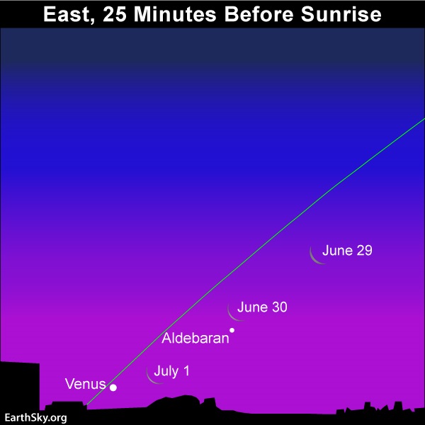
On the morning of July 1 – as seen from around the world – the waning moon is near bright Venus. This very bright planet is also very low in your eastern dawn sky and thus not easy to see. Read more.

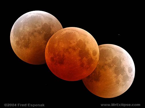
Venus, the brightest planet, looms low in the east before sunrise in early July 2019. Day by day, Venus sinks closer to the sunrise, so this world must contend with the sun’s glare throughout this month. However, if you’re in just the right spot in South America, you can watch Venus pop into view during the total eclipse of the sun on July 2, 2019.

In early July, at mid-northern latitudes, Venus rises less than an hour before sunrise. By the month’s end, that’ll taper to about 20 minutes.

At temperate latitudes in the Southern Hemisphere, Venus rises about 50 minutes before sunup in early July. By the month’s end that’ll decrease to about 10 minutes.

In other words – for all of Earth – Venus will disappear from our sky in early July, assuming you’re looking with your eye alone.

What is happening to Venus? Where’s it going? It’s now fleeing ahead of Earth in the race of the planets around the sun. On August 14, 2019, Venus will reach superior conjunction, when it will be behind the sun as seen from Earth. At that point, it’ll transition from the morning to evening sky. Most of us will begin to see Venus as a bright evening “star” in September.

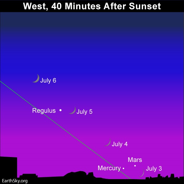
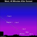
Coming soon! The young evening crescent swings by the planets Mercury and Mars on July 3 and 4, 2019. They’ll be hard to see in the afterglow of sunset; you’ll definitely want your binoculars. Read more.

Mercury starts off the month rather close to Mars on the sky’s dome. Your best chance of catching them is early in the month, when these two worlds are out for a maximum amount of time after sunset. On July 3 and 4, 2019, the young crescent moon will be in the vicinity of Mercury and Mars. But all three celestial bodies – the moon, Mercury and Mars – will have to contend with the glow of sunset, so have binoculars handy.

Click here for recommended sky almanacs providing you with the setting times for Mercury and Mars in your sky.

Day by day, however, these two worlds sink closer to the sunset, with Mercury doing so at a much faster pace than Mars. Mercury moves faster than Mars in orbit, and it moves faster in our sky as well. That’s why the early stargazers named Mercury for their fleet-footed messenger god.

Mercury will meet up with the sun, at inferior conjunction, on July 21, 2019. In the days before and after Mercury’s July 21 conjunction, skilled observers with telescopes will be able to view the planet as a thin crescent world. July 21 will also mark Mercury’s transition out of the evening sky and into the morning sky.

Mars will meet up with the sun, at superior conjunction, on September 2, 2019. For at least six weeks or so on either side of that date, Mars will be absent from our sky, lost in the sun’s glare.

By the way, at this upcoming conjunction, Mercury will swing to the south of the sun’s disk as seen from Earth. But when Mercury reaches its next inferior conjunction on November 11, 2019, the innermost planet will swing directly in front of the sun, to stage a transit of Mercury. Transits of Mercury happen more frequently than transits of Venus; they happen 13 or 14 times per century. The last transit of Mercury happened on May 9, 2016, and – after the one on this upcoming November 11 – the next Mercury transit won’t be until November 13, 2032.

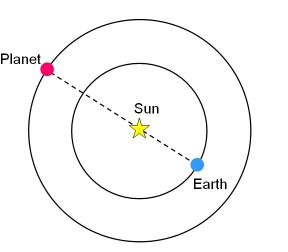
Here’s a superior conjunction. The planet sweeps behind the sun as seen from Earth. Image via COSMOS.

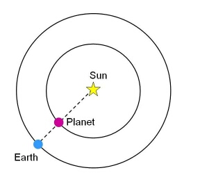
Here’s an inferior conjunction. The planet sweeps between the Earth and sun. As seen from Earth, only Venus and Mercury can have inferior conjunctions. Image via COSMOS.

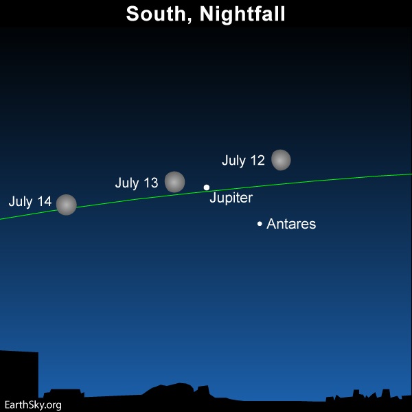
On the evenings of July 12, 13 and 14, 2019, watch for the bright waxing gibbous moon to swing by the giant planet Jupiter. Read more.

Jupiter – the second-brightest planet after Venus – reigns supreme in the July 2019 nighttime sky. Venus is mostly lost in the glare of sunrise throughout July. Jupiter, on the other hand, pops out in the eastern sky at dusk and stays out nearly all night. Jupiter is very bright, brighter than any star. Still not sure? See the moon in Jupiter’s vicinity for several days, centered on or near July 13.

Jupiter’s yearly opposition was June 10, 2019, when this planet lit up the night sky from dusk until dawn. Now, since Jupiter is already in the east when night begins, it doesn’t make it until dawn. From around the world in early July, Jupiter sets about 1 1/2 hours before sunrise (approximate beginning of astronomical twilight). By the end of the month, Jupiter will set beneath the southwest horizon about two hours before the start of astronomical twilight.

Click here to find out when astronomical twilight comes to your sky, remembering to check the astronomical twilight box.

That bright ruddy star rather close to Jupiter on our sky’s dome this year is Antares, the Heart of the Scorpion in the constellation Scorpius. Throughout 2019, Jupiter can be seen to “wander” relative to this zodiac star. In other words, in the first three months of 2019, Jupiter was traveling eastward, away from Antares. But starting on April 10, 2019, Jupiter appeared to reverse course, moving toward Antares. For four months (April 10 to August 11, 2019), Jupiter will be traveling in retrograde (or westward), closing the gap between itself and the star Antares. Midway through this retrograde – on June 10, 2019 – Jupiter reached opposition.

Can’t find Saturn? The almost-full moon pairs up with it as darkness falls on July 15, 2019. Read more.

Saturn reaches opposition on July 9, 2019. At opposition, Saturn rises in the east around sunset, climbs highest up for the night at midnight (midway between sunset and sunrise) and sets in the west around sunrise. Opposition happens when Earth in its orbit swings between the sun and Saturn. Our two worlds are close now, and Saturn, in turn, shines at its brightest best in Earth’s sky.

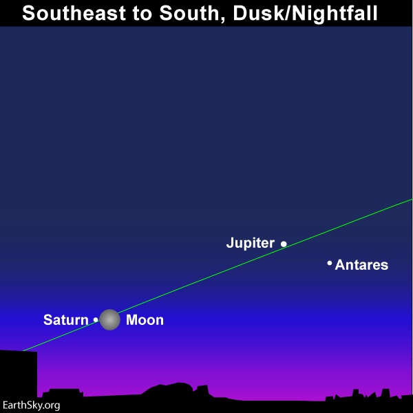
Watch for the bright moon to couple up with Saturn on or near July 15, as shown on the sky chart above. If you’re in just the right spot in South America, you can actually watch the moon occult (cover over) Saturn on the night of July 15-16, 2019.

Don’t mistake Saturn for the more brilliant planet Jupiter. At nightfall and early evening in July 2019, Saturn shines well below Jupiter and quite close to the southeast horizon. Saturn, although somewhat brighter than a 1st-magnitude star, pales in contrast to the king planet. Jupiter, the fourth-brightest celestial object after the sun, moon and Venus, respectively, outshines Saturn by some 11 times.

In early July 2019, Saturn rises about 1/2 hour after sunset. At opposition on July 9, Saturn rises as the sun sets.

By the month’s end, Saturn comes up roughly 1 1/2 hours before sunset, though the exact figure varies somewhat, depending on your latitude.

Viewing Saturn’s rings soon? Read me 1st

Here’s an opposition. It happens when Earth flies between a planet and the sun. This happens yearly for most of the outer planets (except Mars). Note that the image is not to scale. Saturn is about 9.5 times the Earth’s distance from the sun. Earth goes between the sun and Saturn once a year, 2 weeks later each year. Image via Heavens Above.

What do we mean by bright planet? By bright planet, we mean any solar system planet that is easily visible without an optical aid and that has been watched by our ancestors since time immemorial. In their outward order from the sun, the five bright planets are Mercury, Venus, Mars, Jupiter and Saturn. These planets actually do appear bright in our sky. They are typically as bright as – or brighter than – the brightest stars. Plus, these relatively nearby worlds tend to shine with a steadier light than the distant, twinkling stars. You can spot them, and come to know them as faithful friends, if you try.

Skywatcher, by Predrag Agatonovic.

Bottom line: In July 2019, two planets – Jupiter and Saturn – are easy to see throughout the month. They both come out at nightfall and are out nearly all night long. Mercury and Mars lurk low in the afterglow of sunset, whereas Venus sits deeply in the glare of morning dawn. Click here for recommended almanacs; they can help you know when the planets rise and set in your sky.

Don’t miss anything. Subscribe to EarthSky News by email

Visit EarthSky’s Best Places to Stargaze, and recommend a place we can all enjoy. Zoom out for worldwide map.

Help EarthSky keep going! Donate now.

Post your planet photos at EarthSky Community Photos

from EarthSky https://ift.tt/1YD00CF

Click the name of a planet to learn more about its visibility in July 2019: Venus, Jupiter, Saturn, Mars and Mercury.

On the morning of July 1 – as seen from around the world – the waning moon is near bright Venus. This very bright planet is also very low in your eastern dawn sky and thus not easy to see. Read more.

Venus, the brightest planet, looms low in the east before sunrise in early July 2019. Day by day, Venus sinks closer to the sunrise, so this world must contend with the sun’s glare throughout this month. However, if you’re in just the right spot in South America, you can watch Venus pop into view during the total eclipse of the sun on July 2, 2019.

In early July, at mid-northern latitudes, Venus rises less than an hour before sunrise. By the month’s end, that’ll taper to about 20 minutes.

At temperate latitudes in the Southern Hemisphere, Venus rises about 50 minutes before sunup in early July. By the month’s end that’ll decrease to about 10 minutes.

In other words – for all of Earth – Venus will disappear from our sky in early July, assuming you’re looking with your eye alone.

What is happening to Venus? Where’s it going? It’s now fleeing ahead of Earth in the race of the planets around the sun. On August 14, 2019, Venus will reach superior conjunction, when it will be behind the sun as seen from Earth. At that point, it’ll transition from the morning to evening sky. Most of us will begin to see Venus as a bright evening “star” in September.

Coming soon! The young evening crescent swings by the planets Mercury and Mars on July 3 and 4, 2019. They’ll be hard to see in the afterglow of sunset; you’ll definitely want your binoculars. Read more.

Mercury starts off the month rather close to Mars on the sky’s dome. Your best chance of catching them is early in the month, when these two worlds are out for a maximum amount of time after sunset. On July 3 and 4, 2019, the young crescent moon will be in the vicinity of Mercury and Mars. But all three celestial bodies – the moon, Mercury and Mars – will have to contend with the glow of sunset, so have binoculars handy.

Click here for recommended sky almanacs providing you with the setting times for Mercury and Mars in your sky.

Day by day, however, these two worlds sink closer to the sunset, with Mercury doing so at a much faster pace than Mars. Mercury moves faster than Mars in orbit, and it moves faster in our sky as well. That’s why the early stargazers named Mercury for their fleet-footed messenger god.

Mercury will meet up with the sun, at inferior conjunction, on July 21, 2019. In the days before and after Mercury’s July 21 conjunction, skilled observers with telescopes will be able to view the planet as a thin crescent world. July 21 will also mark Mercury’s transition out of the evening sky and into the morning sky.

Mars will meet up with the sun, at superior conjunction, on September 2, 2019. For at least six weeks or so on either side of that date, Mars will be absent from our sky, lost in the sun’s glare.

By the way, at this upcoming conjunction, Mercury will swing to the south of the sun’s disk as seen from Earth. But when Mercury reaches its next inferior conjunction on November 11, 2019, the innermost planet will swing directly in front of the sun, to stage a transit of Mercury. Transits of Mercury happen more frequently than transits of Venus; they happen 13 or 14 times per century. The last transit of Mercury happened on May 9, 2016, and – after the one on this upcoming November 11 – the next Mercury transit won’t be until November 13, 2032.

Here’s a superior conjunction. The planet sweeps behind the sun as seen from Earth. Image via COSMOS.

Here’s an inferior conjunction. The planet sweeps between the Earth and sun. As seen from Earth, only Venus and Mercury can have inferior conjunctions. Image via COSMOS.

On the evenings of July 12, 13 and 14, 2019, watch for the bright waxing gibbous moon to swing by the giant planet Jupiter. Read more.

Jupiter – the second-brightest planet after Venus – reigns supreme in the July 2019 nighttime sky. Venus is mostly lost in the glare of sunrise throughout July. Jupiter, on the other hand, pops out in the eastern sky at dusk and stays out nearly all night. Jupiter is very bright, brighter than any star. Still not sure? See the moon in Jupiter’s vicinity for several days, centered on or near July 13.

Jupiter’s yearly opposition was June 10, 2019, when this planet lit up the night sky from dusk until dawn. Now, since Jupiter is already in the east when night begins, it doesn’t make it until dawn. From around the world in early July, Jupiter sets about 1 1/2 hours before sunrise (approximate beginning of astronomical twilight). By the end of the month, Jupiter will set beneath the southwest horizon about two hours before the start of astronomical twilight.

Click here to find out when astronomical twilight comes to your sky, remembering to check the astronomical twilight box.

That bright ruddy star rather close to Jupiter on our sky’s dome this year is Antares, the Heart of the Scorpion in the constellation Scorpius. Throughout 2019, Jupiter can be seen to “wander” relative to this zodiac star. In other words, in the first three months of 2019, Jupiter was traveling eastward, away from Antares. But starting on April 10, 2019, Jupiter appeared to reverse course, moving toward Antares. For four months (April 10 to August 11, 2019), Jupiter will be traveling in retrograde (or westward), closing the gap between itself and the star Antares. Midway through this retrograde – on June 10, 2019 – Jupiter reached opposition.

Can’t find Saturn? The almost-full moon pairs up with it as darkness falls on July 15, 2019. Read more.

Saturn reaches opposition on July 9, 2019. At opposition, Saturn rises in the east around sunset, climbs highest up for the night at midnight (midway between sunset and sunrise) and sets in the west around sunrise. Opposition happens when Earth in its orbit swings between the sun and Saturn. Our two worlds are close now, and Saturn, in turn, shines at its brightest best in Earth’s sky.

Watch for the bright moon to couple up with Saturn on or near July 15, as shown on the sky chart above. If you’re in just the right spot in South America, you can actually watch the moon occult (cover over) Saturn on the night of July 15-16, 2019.

Don’t mistake Saturn for the more brilliant planet Jupiter. At nightfall and early evening in July 2019, Saturn shines well below Jupiter and quite close to the southeast horizon. Saturn, although somewhat brighter than a 1st-magnitude star, pales in contrast to the king planet. Jupiter, the fourth-brightest celestial object after the sun, moon and Venus, respectively, outshines Saturn by some 11 times.

In early July 2019, Saturn rises about 1/2 hour after sunset. At opposition on July 9, Saturn rises as the sun sets.

By the month’s end, Saturn comes up roughly 1 1/2 hours before sunset, though the exact figure varies somewhat, depending on your latitude.

Viewing Saturn’s rings soon? Read me 1st

Here’s an opposition. It happens when Earth flies between a planet and the sun. This happens yearly for most of the outer planets (except Mars). Note that the image is not to scale. Saturn is about 9.5 times the Earth’s distance from the sun. Earth goes between the sun and Saturn once a year, 2 weeks later each year. Image via Heavens Above.

What do we mean by bright planet? By bright planet, we mean any solar system planet that is easily visible without an optical aid and that has been watched by our ancestors since time immemorial. In their outward order from the sun, the five bright planets are Mercury, Venus, Mars, Jupiter and Saturn. These planets actually do appear bright in our sky. They are typically as bright as – or brighter than – the brightest stars. Plus, these relatively nearby worlds tend to shine with a steadier light than the distant, twinkling stars. You can spot them, and come to know them as faithful friends, if you try.

Skywatcher, by Predrag Agatonovic.

Bottom line: In July 2019, two planets – Jupiter and Saturn – are easy to see throughout the month. They both come out at nightfall and are out nearly all night long. Mercury and Mars lurk low in the afterglow of sunset, whereas Venus sits deeply in the glare of morning dawn. Click here for recommended almanacs; they can help you know when the planets rise and set in your sky.

Don’t miss anything. Subscribe to EarthSky News by email

Visit EarthSky’s Best Places to Stargaze, and recommend a place we can all enjoy. Zoom out for worldwide map.

Help EarthSky keep going! Donate now.

Post your planet photos at EarthSky Community Photos

from EarthSky https://ift.tt/1YD00CF

Why no eclipse every full and new moon?

Total lunar eclipse composite image by Fred Espenak.

A lunar eclipse happens when the Earth, sun and moon align in space, with Earth between the sun and moon. At such times, Earth’s shadow falls on the full moon, darkening the moon’s face and – at mid-eclipse – usually turning it a coppery red.

A solar eclipse happens at the opposite phase of the moon – new moon – when the moon passes between the sun and Earth.

Why aren’t there eclipses at every full and new moon?

The moon takes about a month to orbit around the Earth. If the moon orbited in the same plane as the ecliptic – Earth’s orbital plane – we would have a minimum of two eclipses every month. There’d be an eclipse of the moon at every full moon. And, one fortnight (approximately two weeks) later there’d be an eclipse of the sun at new moon for a total of at least 24 eclipses every year.

But the moon’s orbit is inclined to Earth’s orbit by about five degrees. Twice a month the moon intersects the ecliptic – Earth’s orbital plane – at points called nodes. If the moon is going from south to north in its orbit, it’s called an ascending node. If the moon is going from north to south, it’s a descending node. If the full moon or new moon is appreciably close to one of these nodes, then an eclipse is not only possible – but inevitable.

Coming up…Total lunar eclipse of July 2, 2019

Visit EarthSky’s Best Places to Stargaze to find an eclipse-viewing location

Post your eclipse photo to EarthSky Community Photos

The plane of the moon’s orbit is inclined at 5 degrees to the ecliptic (Earth’s orbital plane). In this diagram, the ecliptic is portrayed as the sun’s apparent annual path through the constellations of the zodiac. The moon’s orbit intersects the ecliptic at two points called nodes (N1 and N2).

Solar and lunar eclipses always come in pairs, with one following the other in a period of one fortnight (approximately two weeks). For example, in January 2019, the descending node partial solar eclipse on January 6 was followed by the ascending node total lunar eclipse on January 21.

Then exactly six lunar months (six new moons) after the descending node partial solar eclipse on January 6, there’s an ascending node total solar eclipse on July 2. One fortnight after this ascending node July 2 total solar eclipse, there will be a descending node partial lunar eclipse on July 16.

Then exactly six lunar months (six new moons) after the ascending node total solar eclipse of July 2, the final eclipse of 2019 will present a descending node annular solar eclipse on December 26. One fortnight later, the first eclipse of 2020 will fall on January 10, 2020, to feature an ascending node and hard-to-see penumbral lunar eclipse.

Read more: Dates of solar and lunar eclipses in 2019

More often than not, two eclipses – one solar and one lunar – occur in one eclipse season, a period lasting approximately 34 to 35 days. Sometimes, though, when the initial eclipse happens sufficiently early in the eclipse season, there can be three eclipses in one eclipse season (two solar and one lunar, or two lunar and one solar). The last time this happened was in 2018 (solar/lunar/solar), and the next time will be in 2020 (lunar/solar/lunar).

Read more: How often are there 3 eclipses in a month?

This year, in 2019, the middle of the eclipse season happens on January 17, July 10 and December 30. At the middle of an eclipse season, which recurs in periods of about 173 days, the lunar nodes are in exact alignment with the Earth and sun.

The video below explains why a pair of eclipses happens when the new moon and full moon are closely aligned with the lunar nodes.

There might be some unfamiliar words in this video, including ecliptic and node. The ecliptic is the plane of Earth’s orbit around the sun. The moon’s orbit is inclined to the plane of the ecliptic. The nodes are the two points where the moon’s orbit and the ecliptic intersect.

Relative to the moon’s nodes, the moon’s phases recur about 30 degrees farther eastward (counterclockwise) along the zodiac each month. So the next pair of eclipses won’t be forthcoming for nearly another six calendar months (6 x 30 degrees = 180 degrees), to fall on December 26, 2019, and January 10, 2020.

Node passages of the moon: 2001 to 2100

Phases of the moon: 2001 to 2100

The following new moon and full moon happen again nearly 30 degrees farther eastward as measured by the constellations of the zodiac in about 29.5 days. But the moon returns to its node a good two days earlier than that, or in about 27.2 days. After the eclipses of July 2 and 16, 2019, it’ll be a waning crescent moon (not a new moon) that crosses the moon’s ascending node on July 30, 2019, and a waxing gibbous moon (not a full moon) that crosses the moon’s descending node on August 12, 2019.

A heliocentric or sun-centered view of eclipses in 2019. Earth-moon orbit shown at new and full moon dates. Sizes of Earth, moon, sun very exaggerated. The plane of the moon’s orbit is in blue, with the dark-blue half to the north of the ecliptic, and the light-blue half to the south of the ecliptic. The line dividing the dark-blue and light-blue sides depicts the line of nodes. There’s an eclipse if the moon is full or new when it is in or near the ecliptic or sun-Earth plane. This year there are 5 eclipses, instead of the most usual 4, because a 3rd eclipse season begins before the end of the year. Illustration via Guy Ottewell.

Even though the moon’s orbit is inclined to that of Earth – and even though there’s not an eclipse with every new and full moon – there are more eclipses than you might think.

There are from four to seven eclipses every year. Some are solar, some are lunar, some are total, and some are partial. All are marvelous to behold – a reminder that we live on a planet – a chance to experience falling in line with great worlds in space!

Photo via pizzodisevo.

Bottom line: There’s no eclipse at every full moon and new moon because the moon’s orbit is inclined to Earth’s orbit by about five degrees. Most of the time, the sun, Earth and moon don’t line up precisely enough to cause an eclipse. But sometimes, more often than you might expect, they do!

Donate: It means the world to us

EarthSky lunar calendars are cool! They make great gifts. Order now. Going fast!

from EarthSky https://ift.tt/2XfOwtU

Total lunar eclipse composite image by Fred Espenak.

A lunar eclipse happens when the Earth, sun and moon align in space, with Earth between the sun and moon. At such times, Earth’s shadow falls on the full moon, darkening the moon’s face and – at mid-eclipse – usually turning it a coppery red.

A solar eclipse happens at the opposite phase of the moon – new moon – when the moon passes between the sun and Earth.

Why aren’t there eclipses at every full and new moon?

The moon takes about a month to orbit around the Earth. If the moon orbited in the same plane as the ecliptic – Earth’s orbital plane – we would have a minimum of two eclipses every month. There’d be an eclipse of the moon at every full moon. And, one fortnight (approximately two weeks) later there’d be an eclipse of the sun at new moon for a total of at least 24 eclipses every year.

But the moon’s orbit is inclined to Earth’s orbit by about five degrees. Twice a month the moon intersects the ecliptic – Earth’s orbital plane – at points called nodes. If the moon is going from south to north in its orbit, it’s called an ascending node. If the moon is going from north to south, it’s a descending node. If the full moon or new moon is appreciably close to one of these nodes, then an eclipse is not only possible – but inevitable.

Coming up…Total lunar eclipse of July 2, 2019

Visit EarthSky’s Best Places to Stargaze to find an eclipse-viewing location

Post your eclipse photo to EarthSky Community Photos

The plane of the moon’s orbit is inclined at 5 degrees to the ecliptic (Earth’s orbital plane). In this diagram, the ecliptic is portrayed as the sun’s apparent annual path through the constellations of the zodiac. The moon’s orbit intersects the ecliptic at two points called nodes (N1 and N2).

Solar and lunar eclipses always come in pairs, with one following the other in a period of one fortnight (approximately two weeks). For example, in January 2019, the descending node partial solar eclipse on January 6 was followed by the ascending node total lunar eclipse on January 21.

Then exactly six lunar months (six new moons) after the descending node partial solar eclipse on January 6, there’s an ascending node total solar eclipse on July 2. One fortnight after this ascending node July 2 total solar eclipse, there will be a descending node partial lunar eclipse on July 16.

Then exactly six lunar months (six new moons) after the ascending node total solar eclipse of July 2, the final eclipse of 2019 will present a descending node annular solar eclipse on December 26. One fortnight later, the first eclipse of 2020 will fall on January 10, 2020, to feature an ascending node and hard-to-see penumbral lunar eclipse.

Read more: Dates of solar and lunar eclipses in 2019

More often than not, two eclipses – one solar and one lunar – occur in one eclipse season, a period lasting approximately 34 to 35 days. Sometimes, though, when the initial eclipse happens sufficiently early in the eclipse season, there can be three eclipses in one eclipse season (two solar and one lunar, or two lunar and one solar). The last time this happened was in 2018 (solar/lunar/solar), and the next time will be in 2020 (lunar/solar/lunar).

Read more: How often are there 3 eclipses in a month?

This year, in 2019, the middle of the eclipse season happens on January 17, July 10 and December 30. At the middle of an eclipse season, which recurs in periods of about 173 days, the lunar nodes are in exact alignment with the Earth and sun.

The video below explains why a pair of eclipses happens when the new moon and full moon are closely aligned with the lunar nodes.

There might be some unfamiliar words in this video, including ecliptic and node. The ecliptic is the plane of Earth’s orbit around the sun. The moon’s orbit is inclined to the plane of the ecliptic. The nodes are the two points where the moon’s orbit and the ecliptic intersect.

Relative to the moon’s nodes, the moon’s phases recur about 30 degrees farther eastward (counterclockwise) along the zodiac each month. So the next pair of eclipses won’t be forthcoming for nearly another six calendar months (6 x 30 degrees = 180 degrees), to fall on December 26, 2019, and January 10, 2020.

Node passages of the moon: 2001 to 2100

Phases of the moon: 2001 to 2100

The following new moon and full moon happen again nearly 30 degrees farther eastward as measured by the constellations of the zodiac in about 29.5 days. But the moon returns to its node a good two days earlier than that, or in about 27.2 days. After the eclipses of July 2 and 16, 2019, it’ll be a waning crescent moon (not a new moon) that crosses the moon’s ascending node on July 30, 2019, and a waxing gibbous moon (not a full moon) that crosses the moon’s descending node on August 12, 2019.

A heliocentric or sun-centered view of eclipses in 2019. Earth-moon orbit shown at new and full moon dates. Sizes of Earth, moon, sun very exaggerated. The plane of the moon’s orbit is in blue, with the dark-blue half to the north of the ecliptic, and the light-blue half to the south of the ecliptic. The line dividing the dark-blue and light-blue sides depicts the line of nodes. There’s an eclipse if the moon is full or new when it is in or near the ecliptic or sun-Earth plane. This year there are 5 eclipses, instead of the most usual 4, because a 3rd eclipse season begins before the end of the year. Illustration via Guy Ottewell.

Even though the moon’s orbit is inclined to that of Earth – and even though there’s not an eclipse with every new and full moon – there are more eclipses than you might think.

There are from four to seven eclipses every year. Some are solar, some are lunar, some are total, and some are partial. All are marvelous to behold – a reminder that we live on a planet – a chance to experience falling in line with great worlds in space!

Photo via pizzodisevo.

Bottom line: There’s no eclipse at every full moon and new moon because the moon’s orbit is inclined to Earth’s orbit by about five degrees. Most of the time, the sun, Earth and moon don’t line up precisely enough to cause an eclipse. But sometimes, more often than you might expect, they do!

Donate: It means the world to us

EarthSky lunar calendars are cool! They make great gifts. Order now. Going fast!

from EarthSky https://ift.tt/2XfOwtU