Old moon, Venus, Mercury

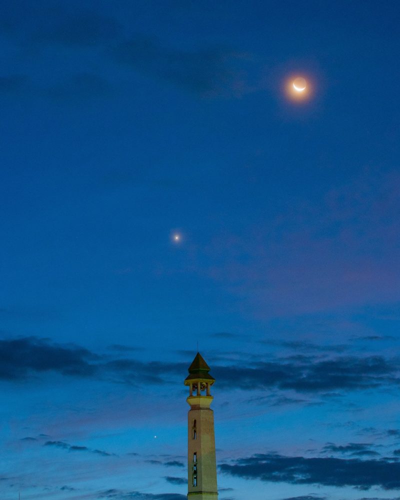
Waning crescent moon with earthshine, Venus and fainter Mercury, in a twilight sky.

View at EarthSky Community Photos. | Asthadi Setyawan in Malang, East Java, Indonesia caught the waning crescent moon, bright Venus and Mercury (lower left) on May 2, 2019. Thank you, Asthadi!


from EarthSky http://bit.ly/2VF1vsl

New moon is May 4

Extremely thin crescent against blue background.

Youngest possible lunar crescent, with the moon’s age being exactly zero when this photo was taken — at the instant of new moon – 07:14 UTC on July 8, 2013. Image by Thierry Legault.

The next new moon falls on May 4, 2019, at 22:45 UTC; translate UTC to your time. This new moon is of interest to Muslims around the world because – in the days following it – the earliest sightings of a young crescent moon in the west after sunset will mark the start of the Islamic holy month of Ramadan.

Read more: When does Ramadan begin in 2019?

New moons can’t be seen, or at least they can’t without special equipment and a lot of moon-watching experience. The photo at the top of this post shows the moon at the instant it became new in July 2013. When the moon is new, it’s most nearly between the Earth and sun for any particular month. There’s a new moon about once a month, because the moon takes about a month to orbit Earth. The moon is nearly between the Earth and sun. In most months, there’s no eclipse because, most of the time, the new moon passes not in front of the sun, but simply near it in our sky.

Either way – in front of the sun or just near it – on the day of new moon, the moon travels across the sky with the sun during the day, hidden in the sun’s glare.

A day or two after each month’s new moon, a slim crescent moon always becomes visible in the west after sunset. In the language of astronomy, this slim crescent is called a young moon by astronomers. Will you see the May young moon after sunset on May 5? More about that in the next paragraph. The exact time of young moon (in this case 22:45 UTC on May 4, 2019) determines your young moon possibilities; it’s rare (but really fun and beautiful) to see a young moon less than 24 hours from new. That’s because the moon needs to be far enough from the sun on the sky’s dome for you to be able to see it. It needs time to move in orbit, to achieve that distance from the sun in our sky. The time of year makes a difference, too. The months around your spring equinox (March for the Northern Hemisphere, September for the Southern Hemisphere) provide your best chance to see your youngest moons.

The time of this month’s new moon – 22:45 UTC on May 4, 2019 – translates to 6:45 p.m. EDT on May 4. That’s the new moon instant for the east coast of the North America. The moon sets with the sun that day; you won’t see it from anywhere on Earth.

The next day – May 5, from, for example, New York City – the moon sets less than an hour after sunset. So you might see the May 5 young moon from New York (and from anywhere on the east coast of North America), but … wow. Tough observation. You would definitely need to be looking very shortly after sunset, at a very clear western horizon, and using some optical aid. East of there? Europe, Middle East, Africa? Very unlikely you’ll see the young moon May 5 with the eye alone, but telescopes and binoculars might pick it up. West of there? Western North America and islands in the Pacific? Your young moon chances on May 5 are better.

Most likely, for most of us around the world, we’ll see this month’s young moon with the eye alone beginning on May 6. From New York City, for example, on May 6 the moon sets about two hours after the sun.

New moons, and young moons, are fascinating to many. The Farmer’s Almanac, for example, still offers information on gardening by the moon. And many cultures have holidays based on moon phases.

Chart of waxing crescent moon from night to night, May 6-8, as it passes Mars in the western twilight sky.

Watch for the young moon to sweep past the planet Mars around May 6 to May 8, 2019. Read more.

Bottom line: New moon is May 4, 2019, at 22:45 UTC; translate UTC to your time.

Read more: Young moon and Mars after sunset May 6, 7, 8

Read more: 4 keys to understanding moon phases

Read more: EarthSky’s guide to the bright planets

Help EarthSky keep going! Please donate.


from EarthSky http://bit.ly/2WkA18l

Eta Aquariids before dawn May 4, 5, 6

Image at top: Eta Aquariid meteors over the Atacama Desert in 2015, via Yuri Beletsky.

Before dawn these next several mornings – May 4, 5 and 6, 2019 – watch for meteors in the annual Eta Aquariid meteor shower to streak across the heavens in an inky dark sky unmarred by moonlight. We expect the morning of May 5 to showcase the peak number of meteors. But try the mornings before and after as well, as this meteor shower has a relatively broad peak.

Although the shower can be seen from all parts of Earth, the Eta Aquariids are especially fine from Earth’s Southern Hemisphere, and from the more southerly latitudes in the Northern Hemisphere. Appreciably north of 40 degrees north latitude (the latitude of Denver, Colorado; Beijing, China; and Madrid, Spain), the meteors are few and far between. The reason has to do with the time of twilight and sunrise on the various parts of Earth. To learn more, check this post on why more Eta Aquariid meteors are visible in the Southern Hemisphere.

It also helps to know that – as seen from all parts of Earth – the dark hour before dawn typically presents the greatest number of Eta Aquariid meteors.

Want to know when morning dawn first starts to light up your sky? Click here and remember to check the astronomical twilight box.

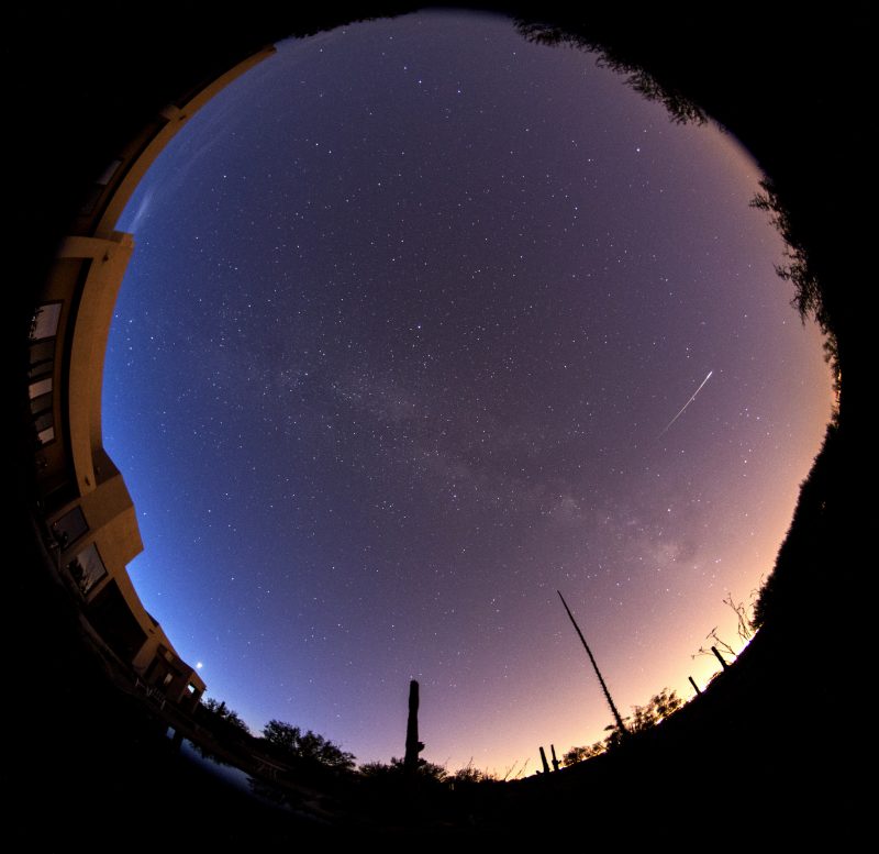
Circular panorama of whole sky, white streak with brighter end, dawn on one side of sky.

Eliot Herman in Tucson caught this meteor during 2017’s Eta Aquariid shower. He said: “… Got this meteor this morning, predawn, really predawn, just minutes before the light wiped out the camera.”

Like most meteors in annual showers, the Eta Aquariids are debris left behind by a comet, and, in this case, it’s a very famous comet indeed. Every year, as Earth passes through the orbital path of Comet Halley, bit and pieces shed by this comet burn up in the Earth’s atmosphere as Eta Aquariid meteors.

May 6, 2017 – Eta Aquariid captured at Mount Bromo (4K timelapse) from Justin Ng Photo on Vimeo.

Under ideal conditions, the Eta Aquariid meteor shower produces up to 20 to 40 meteors per hour. If you’re in the Southern Hemisphere, and you have a very dark sky, you might see that many since this year, in 2019, there is no moon to ruin the show.

And, as always for meteor-watching, be sure to avoid city lights …

You don’t need to find the radiant of the Eta Aquariid shower to watch this meteor shower. But if you’re interested in locating it, use the Great Square of Pegasus to star-hop to the radiant of the Eta Aquariid meteor shower. Read more.

Bottom line: In 2019, the Eta Aquariid meteor shower produces the most meteors before dawn on May 5 in inky dark skies unmarred by moonlight.

Read more: Where’s the radiant point for the Eta Aquariid meteor shower?

Read more: Everything you need to know: Eta Aquariid meteor shower

Read more: EarthSky’s meteor shower guide for 2019


from EarthSky http://bit.ly/2ZRtS5I

Climate change could cost the U.S. economy hundreds of billions a year by 2090

This is a re-post from Yale Climate Connections

A newly-published peer-reviewed analysis of climate change impacts across broad sectors of the U.S. economy provides what may be the most comprehensive economic assessment to date of those costs.

The April report in the journal Nature Climate Change is a condensed version of the Environmental Protection Agency’s 2017 Climate Change Impacts and Risk Analysis report. That analysis was used to help inform the Fourth National Climate Assessment Report published in late 2018.

Written by two EPA professional staffers – but with the standard caveat that it represents their views, and not necessarily those of the agency – the research addressed in the April report considers two global warming scenarios: Representative Concentration Pathway (RCP) 4.5 and 8.5, numbered to correspond to the global energy imbalance (in Watts per square meter) created by the increased greenhouse effect in the two scenarios.

RCP4.5 would lead to about 2.8°C (5°F) warming of global surface temperatures above pre-industrial levels by the year 2100. Limiting global warming to that degree would require more aggressive international climate policies than are in place today, but would nevertheless miss the 2015 Paris climate agreement targets of 2, and ideally of 1.5, degrees C. Continuing emission under the RCP8.5 approach would lead to about 4.5°C (8°F) warming by the end of the century, which is close to a worst-case scenario in which international policies do not slow global fossil fuel use and carbon pollution.

The Nature Climate Change analysis – by EPA scientists Jeremy Martinich and Allison Crimmins – examines 22 different climate economic impacts related to health, infrastructure, electricity, water resources, agriculture, and ecosystems. The bottom line conclusion: by the year 2090, impacts on those 22 economic sectors in the U.S. would cost about $224 billion more per year if we follow the RCP8.5 pathway than if we achieve the RCP4.5 pathway. The authors’ report comes with an important caveat:

only a small portion of the impacts of climate change are estimated, and therefore this Technical Report captures just a fraction of the potential risks and damages that may be avoided or reduced when comparing the alternative scenarios.

Asked to comment on the new research, economist Frank Ackerman, who was not involved with writing the report, said it is “entirely consistent with the broader hypothesis that climate change, if unmitigated, will have large negative impacts throughout the economy before the end of the century.” Impressed with the large number of impacts analyzed, Ackerman, formerly with Tufts University and now principal economist at Synapse Energy Economics, in Cambridge, Ma., said the report would have benefited had the authors been able to use a consistent base year and discount rate in evaluating all of the different impacts.

How much do we value life?

Health impacts account for about three-quarters of the $224 billion per year total cost difference between the two scenarios. More than one-third of that total is attributed to an increase in heat-related deaths.

To estimate the increased health effects costs, the authors reviewed research detailing extreme heat deaths in 49 American cities that account for about one-third of the U.S. population.

In the high-emissions RCP8.5 scenario, about 9,300 more people in those 49 cities would die each year as a result of increased heat. With adaptation efforts like installing extensive and costly air conditioning, the number of deaths could be limited to 4,300.

In the lower-emissions RCP4.5 scenario, heat-related deaths would increase by about 3,900 per year (5,400 fewer than in RCP8.5), but could be limited to 1,300 with adaptation (3,000 fewer than in RCP8.5).

Those findings raise a thorny question: How to quantify the value and the cost of those lost lives?

The researchers, in their April report, address that question by incorporating the “value of a statistical life” (VSL), which EPA describes in a 2010 guidelines document as follows:

VSL is a summary measure for the dollar value of small changes in mortality risk experienced by a large number of people. VSL estimates are derived from aggregated estimates of individual values for small changes in mortality risks. For example, if 10,000 individuals are each willing to pay $500 for a reduction in risk of 1/10,000, then the value of saving one statistical life equals $500 times 10,000 – or $5 million. Note that this does not mean that any single identifiable life is valued at this amount. Rather, the aggregate value of reducing a collection of small individual risks is, in this case, worth $5 million.

EPA currently uses a VSL of $10 million, which this study’s authors adjust to $15.2 million for 2090. Their report thus estimates that saving 5,400 lives per year in 2090 in RCP4.5 as compared RCP8.5 is valued at $82 billion per year. Including adaptation efforts such as installation of extensive air conditioning, the difference of 3,000 lives yields an additional $46 billion cost for RCP8.5 as compared to RCP4.5, plus the added costs such as those associated with installing the necessary infrastructure like city-wide air conditioning.

Of course, any estimate of the value of life is ethically fraught. The challenge is that humans tend to most easily visualize and focus on economic impacts, but it’s difficult to quantify the costs of many climate change consequences like lost health and lives, trauma and suffering, or species extinctions and reduced biodiversity.

That dilemma brings to mind for some a comment that Robert F. Kennedy made in 1968 about the metric of Gross National Product: “It measures everything in short, except that which makes life worthwhile.”

Health, infrastructure, and other costs

The projected warming will lead also to 910 million more lost labor hours per year in 2090 in RCP8.5 than in RCP4.5 – a difference worth about $75 billion per year. This impact is highest in the Southeast ($24 billion in additional annual lost labor), Midwest ($16 billion), and Southwest ($11 billion), where temperatures are hottest.

Infrastructure is the second-costliest category of climate impacts. Under high-emissions scenario RCP8.5, an additional $26 billion of American coastal property would be lost annually toward the end of the century. That contrasts with the lower-emissions RCP4.5, plus an extra $12 billion per year in road damages. Higher electricity demand for cooling will cost an extra $5.8 billion per year. Flooding will cost an extra $3.8 billion per year, and an additional $2.2 billion in winter sports recreation will be lost in the high-emissions scenario. Lost freshwater fishing will cost another $1.4 billion annually.

One interesting aspect of the April analysis is that the economic impact on the agricultural sector is relatively small, with a nationwide cost difference estimated at $1.3 million per year more in 2090 under scenario RCP8.5 than under RCP4.5.

The Martinich-Crimmins report does not take into consideration impacts of worsening extreme weather events on crops, and it therefore underestimates agricultural losses. The research anticipates that although yields will decline for most staple crops – especially for barley, corn, cotton, and rice, but with the exception of wheat – farmers will adapt by using more farmland, changing the crops they grow, and increasing prices. As a result, most of the climate change impacts on the agricultural sector would be passed on to food consumers, in effect, to everybody.

“There are no regions that escape some mix of adverse impacts,” the authors conclude in their analysis. “Lower emissions, and adaptation in relevant sectors, would result in substantial economic benefits.”

Their study shows that limiting global warming to less than 5°F by the end of the century would save the United States a total of about $10 trillion from these 22 climate impacts as compared to an unabated 8°F warming, in addition to saving hundreds of thousands of American lives over those decades.

Big numbers those, dwarfing the billions that one-time Illinois Republican Senator Everett Dirksen is perhaps mistakenly said to have called “real money.” And that is in the context of the authors’ reminder that “this Technical Report captures just a fraction of the potential risks and damages that may be avoided or reduced” when comparing the two climate change growth scenarios … neither of which would achieve the higher of the two higher temperature global surface temperature averages that are at the heart of the 2015 Paris Climate Agreement agreed to by nearly 200 countries worldwide.


from Skeptical Science http://bit.ly/2GSSBht
New research, April 22-28, 2019

A selection of new climate related research articles is shown below. This post has separate sections for: Climate Change, Climate Change Impacts, Climate Change Mitigation, and Other Papers.

Climate change impacts

Mankind

Impacts of exposure to ambient temperature on burden of disease: a systematic review of epidemiological evidence

Can increased outdoor CO2 concentrations impact on the ventilation and energy in buildings? A case study in Shanghai, China

Global warming to increase flood risk on European railways

Winter tourism under climate change in the Pyrenees and the French Alps: relevance of snowmaking as a technical adaptation (open access)

Adjusting sowing date and cultivar shift improve maize adaption to climate change in China

Cultural ecosystem services provided by flowering of cherry trees under climate change: a case study of the relationship between the periods of flowering and festivals

Predicting high-magnitude, low-frequency crop losses using machine learning: an application to cereal crops in Ethiopia (open access)

Effects of climate change on sugarcane production in the state of Paraíba (Brazil): a panel data approach (1990–2015)

Climate change and variability impacts on grazing herds: Insights from a system dynamics approach for semi‐arid Australian rangelands

Ethology, physiological, and ingestive responses of sheep subjected to different temperatures and salinity levels of water

Adaptations in irrigated agriculture in the Mediterranean region: an overview and spatial analysis of implemented strategies (open access)

Ecological restoration as a strategy for mitigating and adapting to climate change: lessons and challenges from Brazil

Biosphere

Local snow melt and temperature—but not regional sea ice—explain variation in spring phenology in coastal Arctic tundra (open access)

Phytoplankton growth and stoichiometric responses to warming, nutrient addition and grazing depend on lake productivity and cell size

Latitudinal variation in soil nematode communities under climate warming‐related range‐expanding and native plants

Projecting impacts of global climate and land‐use scenarios on plant biodiversity using compositional‐turnover modelling

Altitudinal gradients fail to predict fungal symbiont responses to warming

Contributions of competition and climate on radial growth of Pinus massoniana in subtropics of China

Taxonomy, together with ontogeny and growing conditions, drives needleleaf species’ sensitivity to climate in boreal North America

Streamflow regimes and geologic conditions are more important than water temperature when projecting future crayfish distributions

A semi-analytical snow-free vegetation index for improving estimation of plant phenology in tundra and grassland ecosystems

Species‐specific and temporal scale‐dependent responses of birds to drought

Shrub persistence and increased grass mortality in response to drought in dryland systems

Latitude and daily-weather effects on gobbling activity of wild turkeys in Mississippi

Evidence that the Montseny Mountains are still a good climatic refugium for the southernmost silver fir forest on the Iberian Peninsula

The response of English yew (Taxus baccata L.) to climate change in the Caspian Hyrcanian Mixed Forest ecoregion

Other impacts

River temperature and the thermal-dynamic transport of sediment

Climate change mitigation

Climate change communication

Climate uncertainty and policy making—what do policy makers want to know?

Systems thinking as a pathway to global warming beliefs and attitudes through an ecological worldview

Climate Policy

Language and environmental justice: articulating intersectionality within energy policy deliberations

Can Japan enhance its 2030 greenhouse gas emission reduction targets? Assessment of economic and energy-related assumptions in Japan's NDC

The differentiated impact of emissions trading system based on company size

Energy production

Assessing the evolution of India's power sector to 2050 under different CO2 emissions rights allocation schemes

Coal production and consumption analysis, and forecasting of related carbon emission: evidence from China

The role of local governments in the development of China's solar photovoltaic industry

Emission savings

Reduction of the carbon footprint of college freshman diets after a food-based environmental science course

Investigating CO2 mitigation potentials and the impact of oil price distortion in China's transport sector

Do solar study lamps help children study at night? Evidence from rural India

Climate change

Climate science needs to take risk assessment much more seriously (open access)

Temperature, precipitation, wind

The global warming hiatus has faded away: an analysis of 2014–2016 global surface air temperatures

Changes in the dependence between global precipitation and temperature from observations and model simulations

Present-day status and future projection of spring Eurasian surface air temperature in CMIP5 model simulations

An assessment of recent global atmospheric reanalyses for Antarctic near surface air temperature

Monotone trends in the distribution of climate extremes

The Influence of Mesoscale Atmospheric Circulation on Spitsbergen Air Temperature in Periods of Arctic Warming and Cooling

Declining diurnal temperature range in the North China Plain related to environmental changes

Problems in calculating long-term trends in the upper atmosphere

Effects of deforestation on the onset of the rainy season and the duration of dry spells in southern Amazonia

Projected changes in autumn rainfall over West China: results from an ensemble of dynamical downscaling simulations

Near‐surface mean wind in Switzerland: Climatology, climate model evaluation and future scenarios

Extreme events

Climate of the weakly-forced yet high-impact convective storms throughout the Ohio River Valley and Mid-Atlantic United States

Physical understanding of human-induced changes in U.S. hot droughts using equilibrium climate simulations

Characteristics of drought in Southern China under climatic warming, the risk, and countermeasures for prevention and control

Forcings and feedbacks

Anthropogenic aerosols, greenhouse gases and the uptake, transport and storage of excess heat in the climate system

Evaluating climate model simulations of the radiative forcing and radiative response at the Earth’s surface

The Interdecadal Change of Summer Water Vapor over the Tibetan Plateau and Associated Mechanisms

Cryosphere

Uncertainty quantification of the multi-centennial response of the Antarctic ice sheet to climate change (open access)

A new 200‐year spatial reconstruction of West Antarctic surface mass balance

Non-uniform contribution of internal variability to recent Arctic sea ice loss

Northern Hemisphere permafrost map based on TTOP modelling for 2000–2016 at 1 km2 scale

Hydrosphere

Assessment of time of emergence of anthropogenic deoxygenation and warming: insights from a CESM simulation from 850 to 2100 CE (open access)

Regime shift of global oceanic evaporation in the late 1990s using OAFlux dataset

Atmospheric and oceanic circulation

Observation-based estimate of global and basin ocean meridional heat transport time series

Identifying strong signals between low‐frequency climate oscillations and annual precipitation using long‐window correlation analysis

How strong is influence of the tropics and midlatitudes on the Arctic atmospheric circulation and climate change?

Carbon and nitrogen cycles

Characteristics of annual greenhouse gas flux and NO release from alpine meadow and forest on the eastern Tibetan Plateau

Regime shifts of Mediterranean forest carbon uptake and reduced resilience driven by multidecadal ocean surface temperatures

Other papers

Palaeoclimatology

A 2917-year tree-ring-based reconstruction of precipitation for the Buerhanbuda Mts., southeastern Qaidam Basin, China

Arctic vegetation, temperature, and hydrology during Early Eocene transient global warming events

Decadal-scale progression of the onset of Dansgaard–Oeschger warming events (open access)

Challenges associated with the climatic interpretation of water stable isotope records from a highly resolved firn core from Adélie Land, coastal Antarctica (open access)


from Skeptical Science http://bit.ly/2VcjG9p

Arc to Arcturus, spike to Spica

Tonight, look outside in the evening and learn a phrase useful to sky watchers. The phrase is: follow the arc to Arcturus, and drive a spike (or speed on) to Spica. You can use this phrase in any year.

First locate the Big Dipper asterism in the northeastern sky. Then draw an imaginary line following the curve in the Dipper’s handle until you come to a bright orange star. This star is Arcturus in the constellation Bootes, known in skylore as the bear guard.

Arcturus is a giant star with an estimated distance of 37 light-years. It’s special because it’s not moving with the general stream of stars, in the flat disk of the Milky Way galaxy. Instead, Arcturus is cutting perpendicularly through the galaxy’s disk at a tremendous rate of speed … some 100 miles (150 km) per second. Millions of years from now this star will be lost from the view of any future inhabitants of Earth, or at least those who are earthbound and looking with the eye alone.

Now drive a spike or, as some say, speed on to Spica in the constellation Virgo.

Spica in the constellation Virgo looks like one star, but this single point of light is really a multiple star system – with two hot stars orbiting very close together – located an estimated distance of 262 light-years away from Earth.

Sky chart of Spica and Corvus

Here’s another way to verify that you’re looking at Spica, the brightest star in the constellation Virgo.

Bottom line: Follow the arc to Arcturus, and drive a spike to Spica.


Big and Little Dippers: Noticeable in northern sky

Enjoying EarthSky so far? Sign up for our free daily newsletter today!

EarthSky astronomy kits are perfect for beginners. Order today from the EarthSky store

Donate: Your support means the world to us


from EarthSky http://bit.ly/2vEpTeR

Scientists explain mysterious, celestial STEVE

Long beam of pink light shooting into the sky from behind small forested island.

A great example of a STEVE display, taken by Ryan Sault of Alberta Aurora Chasers on the evening of April 10, 2018, in Prince George, British Columbia, Canada.

We’re all aware of, or even familiar with, the aurora borealis – also known as northern lights – those beautiful, shimmering ribbons of light that sometimes dance across the night sky. But there’s another, somewhat lesser-known phenomenon called STEVE (strong thermal emission velocity enhancement) that also puts on fantastic displays, yet isn’t as well understood. Now scientists think they have finally figured out what causes it. They found that STEVE has characteristics similar to those of typical auroras, yet is also uniquely different in how it forms.

Researchers published the new peer-reviewed findings in Geophysical Research Letters on April 16, 2019.

In 2018, a previous study had found that STEVE was a kind of sky glow that was distinct from other auroras, but the researchers didn’t know what was causing it. Whatever the source was, it was seemingly not charged particles hitting Earth’s atmosphere the same way as in typical auroras. But, STEVE could also appear during strong magnetic storms, the kind that produce the brightest displays of auroras: hence, a bit of a puzzle. There were some fantastic displays of STEVE in 2018, which garnered much attention on social media, and caught the attention of researchers.

Unlike other auroras, which are seen as large, brilliant green ribbons, STEVE is a thinner ribbon of pinkish-red or mauve-colored light stretching from east to west, and extending farther south in latitude than other auroras. STEVE displays occur very high up in the atmosphere, at about 15,000 miles (25,000 km) altitude. But, those STEVE displays are also often accompanied by other vertical columns of green light called Picket Fence Auroras that also had not been well understood until now.

Curved pink beam shoots into sky over lake with green aurora in distance.

Another beautiful photo of a STEVE display, near Kamloops, BC, Canada, on September 26, 2016. Image via Dave Markel.

Tall twisted column of pink like beside aurora divided into horizontal pieces.

In this great photo, both a mauve STEVE and a green Picket Fence Aurora display can be seen. Photo taken on May 8, 2016 near Keller, Washington. Image via Rocky Raybell.

Arc of pink like next to green aurora divided into vertical lines.

A stunning Picket Fence Aurora display near Anarchist Mountain, BC, Canada on September 15, 2017. Image via Debra Ceravolo.

Now, the new study has pinpointed two causes of the two phenomena – energetic electrons like those in other auroras, as well as heating of other charged particles in the atmosphere – that create both STEVE and Picket Fence Auroras. STEVE is caused by the heating of charged particles – plasma heating – in the upper atmosphere, but Picket Fence Auroras result from mechanisms more similar to typical auroras. As Bea Gallardo-Lacourt, a space physicist at the University of Calgary and co-author of the new study, explained:

Aurora is defined by particle precipitation, electrons and protons actually falling into our atmosphere, whereas the STEVE atmospheric glow comes from heating without particle precipitation. The precipitating electrons that cause the green picket fence are thus aurora, though this occurs outside the auroral zone, so it’s indeed unique.

The researchers were able to come to these conclusions by studying both satellite data and ground images of STEVE events. Data from several satellites were analyzed as the satellites passed above STEVE events in April 2008 and May 2016. That data was then compared to photographs taken by amateur auroral photographers. In the case of the STEVE displays, it was found that charged particles in the ionosphere – in a “flowing river” – collide with each other. The friction produces heat, and the particles emit mauve-colored light as a result. This is similar to how electricity in an incandescent light bulb heats the filament until it glows.

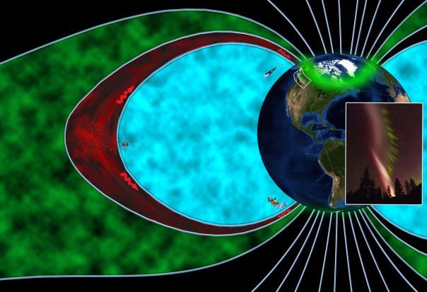
Earth with horse shoe shaped areas radiating from pole to pole.

Artist’s concept of the magnetosphere during a STEVE event, depicting the plasma region which falls into the auroral zone (green), the plasmasphere (blue) and the boundary between them called the plasmapause (red). Image via Emmanuel Masongsong, UCLA/Yukitoshi Nishimura, BU and UCLA.

Picket Fence Auroras, on the other hand, are created by energetic electrons hitting the Earth’s atmosphere from space. This is similar to regular auroras at northern latitudes, except that these particles tend to strike the atmosphere farther south in latitude. The electrons are energized by high-frequency waves moving from Earth’s magnetosphere to the ionosphere; when the electrons are knocked out of the magnetosphere, they create the stripe patterns reminiscent of a picket fence. This process occurs in both hemispheres simultaneously, indicating that the source of the particles is high enough above Earth that the particles can affect both hemispheres at the same time.

STEVE events are also a great way for the public to become involved in auroral research. Photos taken from the ground can provide specific time and location data, which is valuable to scientists. As Toshi Nishimura, a space physicist at Boston University and lead author of the new study, said:

As commercial cameras become more sensitive and increased excitement about the aurora spreads via social media, citizen scientists can act as a ‘mobile sensor network,’ and we are grateful to them for giving us data to analyze.

Aurora borealis, winding curtains of green light over icy sea.

A beautiful example of a “regular” aurora, seen on November 2, 2016, from an airplane flying over northern Canada near the Arctic Circle. Image via Shreenivasan Manievannan.

Learning about exotic phenomena like STEVE and Picket Fence Auroras not only helps scientists understand what causes them, but also how they relate to other auroral phenomena, and what drives such complex processes in Earth’s atmosphere as it interacts with charged particles coming in from space. This is useful not only for understanding the phenomena themselves, but also how to safeguard against possible detrimental effects on radio and GPS signals, which are crucial services in today’s technological world.

Bottom line: Thanks to data from both the public and satellites, scientists have now figured out what causes both STEVE and Picket Fence Aurora phenomena, which are lesser-known but just as beautiful aurora-like sky displays.

Source: Magnetospheric signatures of STEVE: Implication for the magnetospheric energy source and inter-hemispheric conjugacy

Via AGU 100


from EarthSky http://bit.ly/2WiwhV2