A team of scientists have provided the first view of fog as a carrier for microbes. Here, a researcher holds a plate of fungi cultured directly from Namib Desert fog. Image via Juliane Zeidler/Oliver Halsey.
Microbes can catch a ride on fog, says new research. That is, fog can help transfer microorganisms like bacteria, viruses, and fungi, over long distances into new environments, according to the study, published in the journal Science of the Total Environment.
For the study, the researchers measured and compared microbes in fog in two very different, fog-dominated ecosystems: Coastal Maine in the U.S., and the Namib Desert, a hyperarid coastal fog desert on the west coast of southern Africa. They analyzed air samples — both foggy and clear — and rain, filtered to capture bacterial cells at each site, to record the variety and abundance of microorganisms.
Sarah Evans cultures fog microbes from the morning’s fog collection in a makeshift field lab in the Namib Desert. Image via Sarah Fitzpatrick.
Sarah Evans is a Michigan State University biologist and co-lead author of a study. She said in a statement:
Fog droplets were found to be an effective medium for microbial sustenance and transport. At both sites, microbial diversity was higher during and after foggy conditions when compared to clear conditions.
Moisture in fog allows microbes to last longer than they would in dry air. As a result, fog deposits a greater abundance and diversity of microbes onto the land than happens by air alone.
Elias Dueker of Bard College is co-lead author of the study. Dueker said:
When fog rolls in, it can shift the composition of terrestrial airborne microbial communities. And in a fascinating twist, on the journey from the ocean to the land, microbes not only survive, but change during transport. Fog itself is a novel, living ecosystem.
The authors noted that there are also possible health implications for their findings. Fog at both sites contained pathogenic microbes, including suspected plant pathogens and species known to cause respiratory infections in immune-compromised people. This raises concern about the role that fog could play in transporting harmful microbes. Kathleen Weathers, a senior scientist at the Cary Institute of Ecosystem Studies, is a study co-author. She said:
We need a better understanding of fog’s role as a vector for microbes, with special attention to pathogens that threaten health. Warming sea surface temperatures and altered wind regimes are likely to affect fog distribution in many coastal regions.
Bottom line: A new study says that fog is a good carrier of airborne microbes.
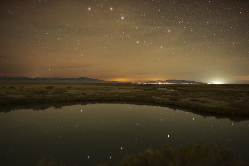
The Big Dipper in October by Marc Toso of the website AncientSkys.com
It’s autumn. There’s a chill in the air, and nights are getting long. Maybe you’ve been standing outside on an autumn evening, looking for the Big Dipper? It’s perhaps the most famous of all star patterns, and – for those at latitudes 41 degrees North or farther north – it’s circumpolar, or always above the northern horizon. If you’re below that latitude, though, you won’t find the Big Dipper in the evening now. In autumn, the Big Dipper is below your horizon during the evening hours.
Want to see it? If you’re in the southern U.S. or a comparable latitude, you’ll want to wait until the hours before dawn. At this time of year, before dawn, you’ll easily see the Big Dipper ascending in the northeast.
To remember the best times to view the Big Dipper in the evening, remember the phrase: spring up and fall down. That’s because the Big Dipper shines way high in the sky on spring evenings but close to the horizon on autumn evenings.
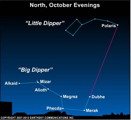
If you’re in the northern U.S., Canada or at a similar latitude, the Big Dipper is circumpolar for you – always above the horizon. These images show the Dipper’s location at roughly 9 p.m. local time April 20 (top), July 20 (west or left), October 20 (bottom) and January 20 (east or right). Just remember “spring up and fall down” for the Dipper’s appearance in our northern sky. It ascends in the northeast on spring evenings, and descends in the northwest on fall evenings. Image via burro.astr.cwru.edu
On autumn evenings, from 41 degrees North latitude, or farther north, the Big Dipper rides low in the north on autumn evenings. As always, the 2 outer stars in the Dipper’s bowl point to Polaris, the North Star.
So you might or might not be able to see the Big Dipper now. But you can think about it. Did you know that the distances of the stars in the Dipper reveal something interesting about them? Five of these seven stars have a physical relationship in space. That’s not always true of patterns on our sky’s dome. Most star patterns are made up of unrelated stars at vastly different distances.
Five of the Big Dipper’s stars – Merak, Mizar, Alioth, Megrez and Phecda – are part of a single star grouping. They probably were born together from a single cloud of gas and dust, and they’re still moving together as a family.
The other two stars in the Dipper – Dubhe and Alkaid – are unrelated to each other and to the other five. Here are the star distances to the Dipper’s stars:
What’s more, Dubhe and Alkaid are moving in an entirely different direction from the other five stars.
And that’s why – millions of years from now – the Big Dipper will have lost its familiar dipper-like shape.
Astronomers have found that the stars of the Big Dipper (excepting the pointer star, Dubhe, and the handle star, Alkaid) belong to an association of stars known as the Ursa Major Moving Cluster. Here are the stars of the Big Dipper, at their various distances from Earth, via AstroPixie.
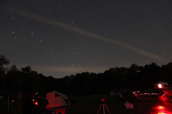
View larger. | Big Dipper on the horizon on an October evening. Kurt Zeppetello caught this image in 2015, while getting set up at the Astronomical Society of New Haven‘s Connecticut Star Party.
Bottom line: If you’re above 41 degrees North latitude, the Big Dipper is circumpolar; it stays in your sky, always, circling around the around the sky’s pole star, Polaris. Below that latitude, the Dipper is below your horizon in the evening in autumn.
The Big Dipper in October by Marc Toso of the website AncientSkys.com
It’s autumn. There’s a chill in the air, and nights are getting long. Maybe you’ve been standing outside on an autumn evening, looking for the Big Dipper? It’s perhaps the most famous of all star patterns, and – for those at latitudes 41 degrees North or farther north – it’s circumpolar, or always above the northern horizon. If you’re below that latitude, though, you won’t find the Big Dipper in the evening now. In autumn, the Big Dipper is below your horizon during the evening hours.
Want to see it? If you’re in the southern U.S. or a comparable latitude, you’ll want to wait until the hours before dawn. At this time of year, before dawn, you’ll easily see the Big Dipper ascending in the northeast.
To remember the best times to view the Big Dipper in the evening, remember the phrase: spring up and fall down. That’s because the Big Dipper shines way high in the sky on spring evenings but close to the horizon on autumn evenings.
If you’re in the northern U.S., Canada or at a similar latitude, the Big Dipper is circumpolar for you – always above the horizon. These images show the Dipper’s location at roughly 9 p.m. local time April 20 (top), July 20 (west or left), October 20 (bottom) and January 20 (east or right). Just remember “spring up and fall down” for the Dipper’s appearance in our northern sky. It ascends in the northeast on spring evenings, and descends in the northwest on fall evenings. Image via burro.astr.cwru.edu
On autumn evenings, from 41 degrees North latitude, or farther north, the Big Dipper rides low in the north on autumn evenings. As always, the 2 outer stars in the Dipper’s bowl point to Polaris, the North Star.
So you might or might not be able to see the Big Dipper now. But you can think about it. Did you know that the distances of the stars in the Dipper reveal something interesting about them? Five of these seven stars have a physical relationship in space. That’s not always true of patterns on our sky’s dome. Most star patterns are made up of unrelated stars at vastly different distances.
Five of the Big Dipper’s stars – Merak, Mizar, Alioth, Megrez and Phecda – are part of a single star grouping. They probably were born together from a single cloud of gas and dust, and they’re still moving together as a family.
The other two stars in the Dipper – Dubhe and Alkaid – are unrelated to each other and to the other five. Here are the star distances to the Dipper’s stars:
What’s more, Dubhe and Alkaid are moving in an entirely different direction from the other five stars.
And that’s why – millions of years from now – the Big Dipper will have lost its familiar dipper-like shape.
Astronomers have found that the stars of the Big Dipper (excepting the pointer star, Dubhe, and the handle star, Alkaid) belong to an association of stars known as the Ursa Major Moving Cluster. Here are the stars of the Big Dipper, at their various distances from Earth, via AstroPixie.
View larger. | Big Dipper on the horizon on an October evening. Kurt Zeppetello caught this image in 2015, while getting set up at the Astronomical Society of New Haven‘s Connecticut Star Party.
Bottom line: If you’re above 41 degrees North latitude, the Big Dipper is circumpolar; it stays in your sky, always, circling around the around the sky’s pole star, Polaris. Below that latitude, the Dipper is below your horizon in the evening in autumn.
Eileen Claffey captured the moon and a fogbow on the morning of September 30, 2018 near Lake Wickaboag in central Massachusetts.
Fogbows are rainbow’s cousins, made by much the same process, but with the small water droplets inside a fog instead of larger raindrops. Because the water droplets in fog are so small, fogbows have only weak colors or are colorless.
Learn more about fogbows (and see great pics!) here.
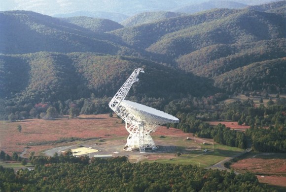
First announced in 2015, Breakthrough Listen is an unprecedented $100 million program – backed by Russian high-tech billionaire Yuri Milner – to listen for signals from an alien intelligence. This massive SETI project is already listening via the Green Bank Telescope in West Virginia and Parkes Telescope in Australia. On October 2, 2018, Breakthrough Listen announced it will also begin listening via the 64 radio dishes of South Africa’s brand new MeerKAT telescope. It made the announcement at the International Astronautical Congress (IAC) in Bremen, Germany, saying it planned to:
… examine a million individual stars – 1,000 times the number of targets in any previous search – in the quietest part of the radio spectrum, monitoring for signs of extraterrestrial technology. With the addition of MeerKAT’s observations to its existing surveys, Listen will operate 24 hours a day, seven days a week.
Yuri Milner commented:
Collaborating with MeerKAT will significantly enhance the capabilities of Breakthrough Listen. This is now a truly global project.
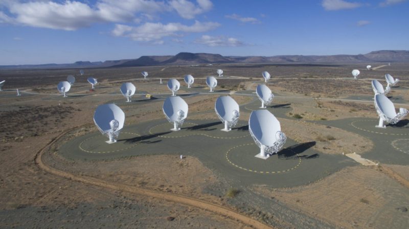
The MeerKAT telescope of the South African Radio Astronomy Observatory is a radio telescope consisting of 64 antennas, located in the remote Karoo Desert of South Africa. Image via SARAO.
Yuri Milner funds Breakthrough Listen. He was an early investor in Facebook and Twitter and has funded other large endeavors, for example, the largest award in the world in the field of Biomedicine and life Sciences, called the Breakthrough Prize. Image via Rusnanotekh.com.
The South African Radio Astronomy Observatory (SARAO) spent part of this year verifying the 64 radio antennas (each 13.5 meters in diameter) of the MeerKAT telescope. SARAO officially inaugurated the telescope in July, 2018.
Breakthrough Listen said its involvement:
…adds the capability to search for technosignatures – signals that indicate the presence of technology on an alien world, and hence provide evidence that intelligent life exists elsewhere.
Scientists and engineers from the University of California, Berkeley SETI Research Center have already installed Breakthrough Listen’s special digital instrumentation at the MeerKAT telescope. The Breakthrough Listen team said its observations will:
… occur in a commensal mode – at the same time as other astrophysics programs. Using sophisticated processing, Breakthrough Listen scientists will digitally point the telescope at targets of interest.
This means that the Breakthrough Listen instrument at MeerKAT will be operating almost continuously, scanning the skies for signs of intelligent life.
The Green Bank telescope in Green Bank, West Virginia is another one of the observatories attempting to eavesdrop on aliens with the help of Breakthrough Listen. Using the Breakthrough Listen digital instrumentation at this telescope, astronomers 3 weeks ago announced they’d found 72 more fast radio bursts from a distant galaxy. Photo via NRAO.
Artist’s concept of an extraterrestrial, via Shutterstock
Bottom line: Yuri Milner’s Breakthrough Listen program has added the new MeerKAT telescope of the South African Radio Astronomy Observatory to its global SETI effort.
from EarthSky https://ift.tt/2P0ZOPu
First announced in 2015, Breakthrough Listen is an unprecedented $100 million program – backed by Russian high-tech billionaire Yuri Milner – to listen for signals from an alien intelligence. This massive SETI project is already listening via the Green Bank Telescope in West Virginia and Parkes Telescope in Australia. On October 2, 2018, Breakthrough Listen announced it will also begin listening via the 64 radio dishes of South Africa’s brand new MeerKAT telescope. It made the announcement at the International Astronautical Congress (IAC) in Bremen, Germany, saying it planned to:
… examine a million individual stars – 1,000 times the number of targets in any previous search – in the quietest part of the radio spectrum, monitoring for signs of extraterrestrial technology. With the addition of MeerKAT’s observations to its existing surveys, Listen will operate 24 hours a day, seven days a week.
Yuri Milner commented:
Collaborating with MeerKAT will significantly enhance the capabilities of Breakthrough Listen. This is now a truly global project.
The MeerKAT telescope of the South African Radio Astronomy Observatory is a radio telescope consisting of 64 antennas, located in the remote Karoo Desert of South Africa. Image via SARAO.
Yuri Milner funds Breakthrough Listen. He was an early investor in Facebook and Twitter and has funded other large endeavors, for example, the largest award in the world in the field of Biomedicine and life Sciences, called the Breakthrough Prize. Image via Rusnanotekh.com.
The South African Radio Astronomy Observatory (SARAO) spent part of this year verifying the 64 radio antennas (each 13.5 meters in diameter) of the MeerKAT telescope. SARAO officially inaugurated the telescope in July, 2018.
Breakthrough Listen said its involvement:
…adds the capability to search for technosignatures – signals that indicate the presence of technology on an alien world, and hence provide evidence that intelligent life exists elsewhere.
Scientists and engineers from the University of California, Berkeley SETI Research Center have already installed Breakthrough Listen’s special digital instrumentation at the MeerKAT telescope. The Breakthrough Listen team said its observations will:
… occur in a commensal mode – at the same time as other astrophysics programs. Using sophisticated processing, Breakthrough Listen scientists will digitally point the telescope at targets of interest.
This means that the Breakthrough Listen instrument at MeerKAT will be operating almost continuously, scanning the skies for signs of intelligent life.
The Green Bank telescope in Green Bank, West Virginia is another one of the observatories attempting to eavesdrop on aliens with the help of Breakthrough Listen. Using the Breakthrough Listen digital instrumentation at this telescope, astronomers 3 weeks ago announced they’d found 72 more fast radio bursts from a distant galaxy. Photo via NRAO.
Artist’s concept of an extraterrestrial, via Shutterstock
Bottom line: Yuri Milner’s Breakthrough Listen program has added the new MeerKAT telescope of the South African Radio Astronomy Observatory to its global SETI effort.
Service members are some of the few professionals who fly into massive storms to collect vital data that lets us know when the storm is coming and how bad it’s going to be.
from https://ift.tt/2QpHBeF
Service members are some of the few professionals who fly into massive storms to collect vital data that lets us know when the storm is coming and how bad it’s going to be.
It’s stunning but true that we know more about the surface of the moon than about the Earth’s ocean floor. Much of what we do know has come from scientific ocean drilling – the systematic collection of core samples from the deep seabed. This revolutionary process began 50 years ago, when the drilling vessel Glomar Challenger sailed into the Gulf of Mexico on August 11, 1968, on the first expedition of the federally funded Deep Sea Drilling Project.
I went on my first scientific ocean drilling expedition in 1980, and since then have participated in six more expeditions to locations including the far North Atlantic and Antarctica’s Weddell Sea. In my lab, my students and I work with core samples from these expeditions. Each of these cores, which are cylinders 31 feet long and 3 inches wide, is like a book whose information is waiting to be translated into words. Holding a newly opened core, filled with rocks and sediment from the Earth’s ocean floor, is like opening a rare treasure chest that records the passage of time in Earth’s history.
Over a half-century, scientific ocean drilling has proved the theory of plate tectonics, created the field of paleoceanography and redefined how we view life on Earth by revealing an enormous variety and volume of life in the deep marine biosphere. And much more remains to be learned.
The scientific drilling ship JOIDES Resolution arrives in Honolulu after successful sea trials and testing of scientific and drilling equipment. Image via IODP.
Technological innovations
Two key innovations made it possible for research ships to take core samples from precise locations in the deep oceans. The first, known as dynamic positioning, enables a 471-foot (144-meter) ship to stay fixed in place while drilling and recovering cores, one on top of the next, often in over 12,000 feet [2 1/2 miles] (3,700 meters [almost 4 km]) of water.
Anchoring isn’t feasible at these depths. Instead, technicians drop a torpedo-shaped instrument called a transponder over the side. A device called a transducer, mounted on the ship’s hull, sends an acoustic signal to the transponder, which replies. Computers on board calculate the distance and angle of this communication. Thrusters on the ship’s hull maneuver the vessel to stay in exactly the same location, countering the forces of currents, wind and waves.
Another challenge arises when drill bits have to be replaced mid-operation. The ocean’s crust is composed of igneous rock that wears bits down long before the desired depth is reached.
The re-entry cone is welded together around the drill pipe, then lowered down the pipe to guide reinsertion before changing drill bits. Image via IODP.
When this happens, the drill crew brings the entire drill pipe to the surface, mounts a new drill bit and returns to the same hole. This requires guiding the pipe into a funnel shaped re-entry cone, less than 15 feet [4.6 m] wide, placed in the bottom of the ocean at the mouth of the drilling hole. The process, which was first accomplished in 1970, is like lowering a long strand of spaghetti into a quarter-inch-wide funnel at the deep end of an Olympic swimming pool.
Confirming plate tectonics
When scientific ocean drilling began in 1968, the theory of plate tectonics was a subject of active debate. One key idea was that new ocean crust was created at ridges in the seafloor, where oceanic plates moved away from each other and magma from earth’s interior welled up between them. According to this theory, crust should be new material at the crest of ocean ridges, and its age should increase with distance from the crest.
The only way to prove this was by analyzing sediment and rock cores. In the winter of 1968-1969, the Glomar Challenger drilled seven sites in the South Atlantic Ocean to the east and west of the Mid-Atlantic ridge. Both the igneous rocks of the ocean floor and overlying sediments aged in perfect agreement with the predictions, confirming that ocean crust was forming at the ridges and plate tectonics was correct.
View complete image. | Part of a core section from the Chicxulub impact crater. It is suevite, a type of rock formed during the impact that contains rock fragments and melted rocks.
Reconstructing earth’s history
The ocean record of Earth’s history is more continuous than geologic formations on land, where erosion and redeposition by wind, water and ice can disrupt the record. In most ocean locations sediment is laid down particle by particle, microfossil by microfossil, and remains in place, eventually succumbing to pressure and turning into rock.
Microfossils (plankton) preserved in sediment are beautiful and informative, even though some are smaller than the width of a human hair. Like larger plant and animal fossils, scientists can use these delicate structures of calcium and silicon to reconstruct past environments.
The resulting acidification of the ocean from the release of carbon into the atmosphere and ocean caused massive dissolution and change in the deep ocean ecosystem.
This episode is an impressive example of the impact of rapid climate warming. The total amount of carbon released during the PETM is estimated to be about equal to the amount that humans will release if we burn all of Earth’s fossil fuel reserves. Yet, an important difference is that the carbon released by the volcanoes and hydrates was at a much slower rate than we are currently releasing fossil fuel. Thus we can expect even more dramatic climate and ecosystem changes unless we stop emitting carbon.
Enhanced scanning electron microscope images of phytoplankton (left, a diatom; right, a coccolithophore). Different phytoplankton species have distinct climatic preferences, which makes them ideal indicators of surface ocean conditions. Image via Dee Breger.
Today scientists from 23 nations are proposing and conducting research through the International Ocean Discovery Program, which uses scientific ocean drilling to recover data from seafloor sediments and rocks and to monitor environments under the ocean floor. Coring is producing new information about plate tectonics, such as the complexities of ocean crust formation, and the diversity of life in the deep oceans.
This research is expensive, and technologically and intellectually intense. But only by exploring the deep sea can we recover the treasures it holds and better understand its beauty and complexity.
The social cost of carbon is a measure of the economic damages caused (via climate change) by each ton of carbon pollution that we produce today. It’s difficult to estimate because of physical, economic, and ethical uncertainties. For example, it’s difficult to predict exactly when various climate tipping points will be triggered, how much their damages will cost, and there’s also a question about how much we value the welfare of future generations (which is incorporated in the choice of ‘discount rate’).
In 2013, the Obama administration set the federal social cost of carbon estimate at $37 per ton of carbon dioxide (up from the previous estimate of $22). That was a conservative estimate – in recent years, research has pegged the value closer to $200 because recent research has shown that global warming slows economic growth, which makes it quite expensive. A majority of economists in a 2015 survey believed the federal estimate was too low, but Republicans have recently been trying to dramatically lower it anyway.
The Republican argument is twofold. First, that we should only consider domestic climate costs (the federal estimate is of global costs, because our carbon pollution doesn’t just hover in the air above America). Second, that instead of trying to stop climate change now, we should just save our money and let future generations pay for its costs (by using a high discount rate).
The social cost of carbon is much higher yet
A new study led by UC San Diego’s Katharine Ricke published in Nature Climate Change found that not only is the global social cost of carbon dramatically higher than the federal estimate – probably between $177 and $805 per ton, most likely $417 – but that the cost to America is around $50 per ton. That’s the second-highest in the world behind India’s $90, and is also higher than the current federal estimate for the global social cost of carbon.
That’s a remarkable conclusion worth repeating. Ricke’s team found that the cost of carbon pollution to just the United States is probably higher than its government’s current estimate of costs to the entire world. And the actual global cost is more than 10 times higher than the federal estimate. And yet Republican politicians think that estimate should be much lower.
The study
I asked Ricke to describe her team’s approach in this study:
To calculate social cost of carbon, you need to answer four questions in sequence:
1. How would the economy change with no climate change (including GHG emissions)?
2. How does the Earth system respond to emissions of carbon dioxide?
3. How does the economy respond to changes in the Earth system?
4. How should we value losses today vs. in (for example) 100 years?
The team answered these questions using four ‘modules’: a socio-economic module to answer the first question, a climate module to address the second, a damages module to investigate the third, and a discounting module to tackle the fourth.
The idea was to combine an approach to analyzing the climate effect of a marginal emission of carbon dioxide that Ken Caldeira and I had recently developed, with a climate damages model described in what was then a working paper by Marshall Burke and collaborators. My co-author Massimo Tavoni pointed out that by combining these two tools, we could produce the first comprehensive, country-level estimates of the social cost of carbon.
The US is at the ideal economic temperature
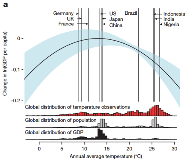
I wrote about the referenced Burke paper in 2015. That study detailed the relationship between a country’s average temperature and its per capita GDP, finding a sweet spot around 13°C (55°F). That’s the optimal temperature for human economic productivity. Economies in countries with lower average temperatures like Canada and Russia would benefit from additional warming, but it would slow economic growth for nations closer to the equator with hotter temperatures.
Global relationship between annual average temperature and change in log gross domestic product (GDP) per capita during 1960–2010 with 90% confidence interval. Illustration: Burke et al. (2015), Nature
The United States is currently right near the peak temperature, whereas many European countries like Germany, the UK, and France are 3–5°C cooler, and a bit below the ideal economic temperature. So, continued global warming is worse for the US economy than Europe’s.
China’s social cost of carbon is lower despite a similar temperature and GDP to America’s because its economy is growing fast, meaning that it would benefit from investing its money now rather than spending it on cutting carbon pollution, at least relative to a more developed country like the US. But China’s social cost of carbon is still about $26 per ton. India’s $90 is the highest because of its combination of a hot climate, high GDP (6th in the world), and anticipated continued growth leading to large future damages.
The social cost of carbon is a measure of the economic damages caused (via climate change) by each ton of carbon pollution that we produce today. It’s difficult to estimate because of physical, economic, and ethical uncertainties. For example, it’s difficult to predict exactly when various climate tipping points will be triggered, how much their damages will cost, and there’s also a question about how much we value the welfare of future generations (which is incorporated in the choice of ‘discount rate’).
In 2013, the Obama administration set the federal social cost of carbon estimate at $37 per ton of carbon dioxide (up from the previous estimate of $22). That was a conservative estimate – in recent years, research has pegged the value closer to $200 because recent research has shown that global warming slows economic growth, which makes it quite expensive. A majority of economists in a 2015 survey believed the federal estimate was too low, but Republicans have recently been trying to dramatically lower it anyway.
The Republican argument is twofold. First, that we should only consider domestic climate costs (the federal estimate is of global costs, because our carbon pollution doesn’t just hover in the air above America). Second, that instead of trying to stop climate change now, we should just save our money and let future generations pay for its costs (by using a high discount rate).
The social cost of carbon is much higher yet
A new study led by UC San Diego’s Katharine Ricke published in Nature Climate Change found that not only is the global social cost of carbon dramatically higher than the federal estimate – probably between $177 and $805 per ton, most likely $417 – but that the cost to America is around $50 per ton. That’s the second-highest in the world behind India’s $90, and is also higher than the current federal estimate for the global social cost of carbon.
That’s a remarkable conclusion worth repeating. Ricke’s team found that the cost of carbon pollution to just the United States is probably higher than its government’s current estimate of costs to the entire world. And the actual global cost is more than 10 times higher than the federal estimate. And yet Republican politicians think that estimate should be much lower.
The study
I asked Ricke to describe her team’s approach in this study:
To calculate social cost of carbon, you need to answer four questions in sequence:
1. How would the economy change with no climate change (including GHG emissions)?
2. How does the Earth system respond to emissions of carbon dioxide?
3. How does the economy respond to changes in the Earth system?
4. How should we value losses today vs. in (for example) 100 years?
The team answered these questions using four ‘modules’: a socio-economic module to answer the first question, a climate module to address the second, a damages module to investigate the third, and a discounting module to tackle the fourth.
The idea was to combine an approach to analyzing the climate effect of a marginal emission of carbon dioxide that Ken Caldeira and I had recently developed, with a climate damages model described in what was then a working paper by Marshall Burke and collaborators. My co-author Massimo Tavoni pointed out that by combining these two tools, we could produce the first comprehensive, country-level estimates of the social cost of carbon.
The US is at the ideal economic temperature
I wrote about the referenced Burke paper in 2015. That study detailed the relationship between a country’s average temperature and its per capita GDP, finding a sweet spot around 13°C (55°F). That’s the optimal temperature for human economic productivity. Economies in countries with lower average temperatures like Canada and Russia would benefit from additional warming, but it would slow economic growth for nations closer to the equator with hotter temperatures.
Global relationship between annual average temperature and change in log gross domestic product (GDP) per capita during 1960–2010 with 90% confidence interval. Illustration: Burke et al. (2015), Nature
The United States is currently right near the peak temperature, whereas many European countries like Germany, the UK, and France are 3–5°C cooler, and a bit below the ideal economic temperature. So, continued global warming is worse for the US economy than Europe’s.
China’s social cost of carbon is lower despite a similar temperature and GDP to America’s because its economy is growing fast, meaning that it would benefit from investing its money now rather than spending it on cutting carbon pollution, at least relative to a more developed country like the US. But China’s social cost of carbon is still about $26 per ton. India’s $90 is the highest because of its combination of a hot climate, high GDP (6th in the world), and anticipated continued growth leading to large future damages.