This is a re-post from Carbon Brief by Daisy Dunne
Limiting global warming to 1.5C above pre-industrial levels rather than 2C could halve the number of vertebrate and plant species facing severe range loss by the end of the century, a study finds.
The analysis of more than 115,000 species finds that keeping warming at 1.5C – which is the aspirational target of the Paris Agreement – instead of 2C could also cut the number of insects facing severe range loss by two-thirds.
However, if countries fail to ramp up their efforts to address climate change, around a quarter of all vertebrates (animals with a spine), half of insects and 44% of plants could face severe range loss, the lead author tells Carbon Brief.
The greatest range losses are expected to occur in some of the world’s biodiversity hotspots, the author adds, including in the Amazon and southern Africa.
Although the findings are significant, the research does not explore all the factors relevant to species survival, including the impact of evolution, another scientist tells Carbon Brief.
Hostile planet
Climate change threatens wildlife in a host of ways. One way is by reducing a species’ geographical range – the extent of the area where it is able to survive.
This can occur when local temperatures become too hot for species to tolerate or when changing rainfall patterns affect the types of food available, for example. As a species’ range contracts, its risk of extinction can increase.
The new study, published in Science, uses a set of global climate models to explore how warming this century could affect the ranges of more than 115,000 species that live on land.
For the analysis, the researchers used four scenarios, including where warming is limited to, in order, 1.5C, 2C, 3.2C (which is the amount of warming anticipated if countries stick to their national pledges to cut emissions) and to 4.5C, the amount of warming expected under a “business as usual” scenario (“RCP8.5”).
The research finds that, if warming is limited to 2C, 8% of vertebrates, 18% of insects and 16% of plants could lose at least half of their current range by 2100.
However, if warming is limited to 1.5C, this risk is halved for vertebrates and plants, and cut by two-thirds for insects.
Unequal losses
The charts below show how future global warming is expected to affect the ranges of invertebrates (A), vertebrates (B) and plants (C) , and also a further breakdown of how warming could affect insects (D), mammals (E) and birds (F).
The x-axis shows temperature rise above pre-industrial levels, while the y-axis shows the proportion of species expected to lose more than half of their range.
On the charts, results for “no dispersal” (yellow) and “realistic dispersal” (blue) are shown. The “realistic dispersal” results consider the ability of animals to move away from their site of birth into new areas, explains lead author Prof Rachel Warren, a researcher of global change and environmental biology at the Tyndall Centre for Climate Change Research. She tells Carbon Brief:
“’No dispersal’ means that we assume the animals don’t move. ‘Dispersal’ means species can move at rates they’ve been observed to move at in response to the climate change that has happened so far.”
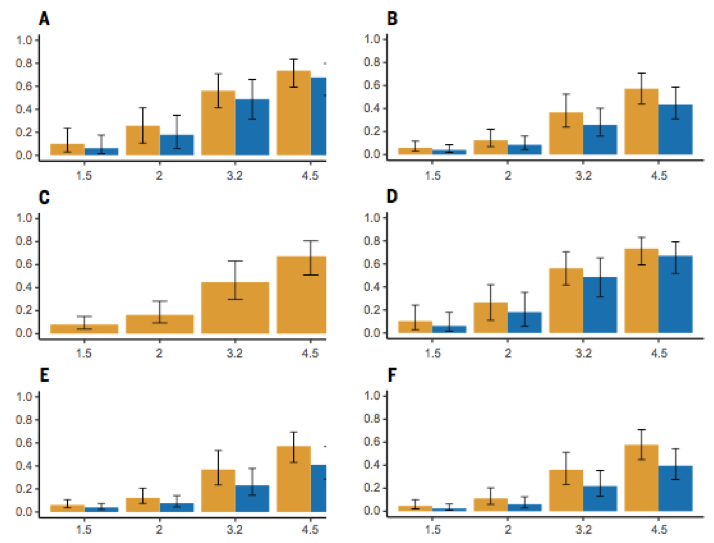
The proportion of species expected to lose more than half of their range by 2100 under different levels of temperature rise. Results are shown for invertebrates (A), vertebrates (B), plants (C), insects (D), mammals (E) and birds (F). Source: Warren et al. (2018)
The results show how invertebrates (A), such as insects, spiders and worms, are expected to lose a larger proportion of their range than vertebrates (B), such as mammals, birds and reptiles.
Insect species at a particularly high risk include key crop pollinators, including bees, hoverflies and blowflies, the research notes. This is due to a range of factors linked to insect physiology and lifestyle, says Warren:
“It is probably because they are ectothermic, which means that their body temperature is controlled externally, not internally, as in humans. Also they have life stages – eggs, larvae, pupae, as well as adults. Each of these stages might be vulnerable to different things, such as eggs drying out if there is too little rainfall.”
Green Hairstreak Butterfly perched on a fern, Devon Coast, UK. Credit: Steve Bloom Images/Alamy Stock Photo.
For mammals (E) and birds (F), risks remain low at 1.5C but grow significantly larger as warming increases, the research finds. Mammals most at risk include critically endangered species such as the black rhino, which also faces significant challenges from habitat loss and poaching.
Warming hotspots
The maps below show how different levels of warming could affect global species diversity for vertebrates. The charts show the proportion of species expected to remain by 2100 – from 90-100% remaining (blue) down to just 0-10% of species remaining (red) – with and without the impact of dispersal.

The proportion of vertebrate species expected to remain in world regions by 2100 under different levels of temperature rise (from top to bottom: 1.5, 2, 3.2, 4.5C). Red shows 0-10% of species remaining while dark blue shows 90-100% remaining. Source: Warren et al. (2018)
The maps reveal that, if future global warming reaches 3.2-4.5C, striking biodiversity loss could occur in some of the world’s wildlife hotspots, including southern Africa and the Amazon – which is home to 30% of the world’s species.
Giraffe in front of Mount Kilimanjaro, Chyulu Hills National Park, Kenya. Credit: Lucas Vallecillos/Alamy Stock Photo.
This could be because temperatures in the tropics and subtropics are relatively consistent from one season to the next, which means resident species are less used to large swings in temperature, says Warren:
“Here in the UK, we can have terrible summers and very nice ones – whereas in the tropics it’s much more predictable. This means that, in temperate lands, species are likely to be buffered against quite large natural climate variability. Whereas in the tropics, as the average climate changes, it could get quickly outside the range of natural variability that species are adapted to.”
Other regions expected to suffer species losses include Australia, the last remaining habitat of marsupials, and the high Arctic, home of the polar bear, the Arctic fox and caribou.
BECCS trade-off
The results show that meeting the Paris Agreement’s aspirational target of limiting warming to 1.5C would bring “substantial benefits” for wildlife, the scientists write in their research paper:
“Successful implementation of the Paris Agreement could lead to substantial benefits for global terrestrial [land] biodiversity…However, restricting warming to 1.5C may be difficult.”
This difficulty lies in the assumption that “negative emissions technologies” will be able to help the world meet the 1.5C target, the researchers say. Most scenarios envisaging how the world could limit warming 1.5C incorporate a negative emissions technology known as bioenergy with carbon capture and storage (BECCS).
Put simply, BECCS involves burning biomass – such as trees and crops – to generate energy and then capturing the resulting CO2 emissions before they are released into the air.
The technology has yet to be demonstrated on a commercial basis, and recent researchshows its potential may be more limited than previously thought.
Even if BECCS is developed on a wide scale, the researchers say, it could pose a significant threat to biodiversity.
That is because large scale BECCS could require up to 18% of the land surface to be converted to biomass plantations, they say, which would drive up competition for land.
This could lead to more deforestation and habitat loss to meet bioenergy and agriculture requirements, they say:
“New studies are exploring scenarios in which BECCS is produced from secondary biofuels, or in which there are dietary changes in humans, resulting in greatly reduced effects of indirect land-use change.”
Survival of the fittest
The study provides “phenomenal coverage” of how climate change could impact biodiversity, says Colin Carlson, a postdoctoral fellow at Georgetown University, who was not involved in the research. Carlson previously published a study looking at the impact of climate change on the world’s parasites. He tells Carbon Brief:
“I expect it’ll be one of the most significant papers in this discipline soon. The focus on climate change mitigation ties into a lot of hot button issues right now – not just Paris, but also alternative solutions for mitigation, like CO2 removal.”
However, the study does not include many of the factors that are key to species survival, says Prof Georgina Mace, director of the Centre for Biodiversity and Environment Research at University College London, who was not involved in the research. She tells Carbon Brief:
“For example, the presence of critical resources, such as food, prey and nest sites; extreme events, pressures from habitat loss, or changes to biotic interactions, often overwhelm climate change effects. So the range loss estimates in this paper have a lot of uncertainty that is not represented.”
The research also does not consider the possibility that some species may be able to evolve new adaptations to cope with climate change, she adds:
“The year 2100 is a long way ahead and species are continuously adapting and evolving; the strong selective pressures mean that many will adapt to deal with climate change. Over this period of time, several hundred generations for many insects, we can expect evolutionary adaptation.”
Warren, R. et al. (2018) The projected effect on insects, vertebrates, and plants of limiting global warming to 1.5C rather than 2C, doi/10.1126/science.aar3646
from Skeptical Science https://ift.tt/2J5NaQ0
This is a re-post from Carbon Brief by Daisy Dunne
Limiting global warming to 1.5C above pre-industrial levels rather than 2C could halve the number of vertebrate and plant species facing severe range loss by the end of the century, a study finds.
The analysis of more than 115,000 species finds that keeping warming at 1.5C – which is the aspirational target of the Paris Agreement – instead of 2C could also cut the number of insects facing severe range loss by two-thirds.
However, if countries fail to ramp up their efforts to address climate change, around a quarter of all vertebrates (animals with a spine), half of insects and 44% of plants could face severe range loss, the lead author tells Carbon Brief.
The greatest range losses are expected to occur in some of the world’s biodiversity hotspots, the author adds, including in the Amazon and southern Africa.
Although the findings are significant, the research does not explore all the factors relevant to species survival, including the impact of evolution, another scientist tells Carbon Brief.
Hostile planet
Climate change threatens wildlife in a host of ways. One way is by reducing a species’ geographical range – the extent of the area where it is able to survive.
This can occur when local temperatures become too hot for species to tolerate or when changing rainfall patterns affect the types of food available, for example. As a species’ range contracts, its risk of extinction can increase.
The new study, published in Science, uses a set of global climate models to explore how warming this century could affect the ranges of more than 115,000 species that live on land.
For the analysis, the researchers used four scenarios, including where warming is limited to, in order, 1.5C, 2C, 3.2C (which is the amount of warming anticipated if countries stick to their national pledges to cut emissions) and to 4.5C, the amount of warming expected under a “business as usual” scenario (“RCP8.5”).
The research finds that, if warming is limited to 2C, 8% of vertebrates, 18% of insects and 16% of plants could lose at least half of their current range by 2100.
However, if warming is limited to 1.5C, this risk is halved for vertebrates and plants, and cut by two-thirds for insects.
Unequal losses
The charts below show how future global warming is expected to affect the ranges of invertebrates (A), vertebrates (B) and plants (C) , and also a further breakdown of how warming could affect insects (D), mammals (E) and birds (F).
The x-axis shows temperature rise above pre-industrial levels, while the y-axis shows the proportion of species expected to lose more than half of their range.
On the charts, results for “no dispersal” (yellow) and “realistic dispersal” (blue) are shown. The “realistic dispersal” results consider the ability of animals to move away from their site of birth into new areas, explains lead author Prof Rachel Warren, a researcher of global change and environmental biology at the Tyndall Centre for Climate Change Research. She tells Carbon Brief:
“’No dispersal’ means that we assume the animals don’t move. ‘Dispersal’ means species can move at rates they’ve been observed to move at in response to the climate change that has happened so far.”
The proportion of species expected to lose more than half of their range by 2100 under different levels of temperature rise. Results are shown for invertebrates (A), vertebrates (B), plants (C), insects (D), mammals (E) and birds (F). Source: Warren et al. (2018)
The results show how invertebrates (A), such as insects, spiders and worms, are expected to lose a larger proportion of their range than vertebrates (B), such as mammals, birds and reptiles.
Insect species at a particularly high risk include key crop pollinators, including bees, hoverflies and blowflies, the research notes. This is due to a range of factors linked to insect physiology and lifestyle, says Warren:
“It is probably because they are ectothermic, which means that their body temperature is controlled externally, not internally, as in humans. Also they have life stages – eggs, larvae, pupae, as well as adults. Each of these stages might be vulnerable to different things, such as eggs drying out if there is too little rainfall.”
Green Hairstreak Butterfly perched on a fern, Devon Coast, UK. Credit: Steve Bloom Images/Alamy Stock Photo.
For mammals (E) and birds (F), risks remain low at 1.5C but grow significantly larger as warming increases, the research finds. Mammals most at risk include critically endangered species such as the black rhino, which also faces significant challenges from habitat loss and poaching.
Warming hotspots
The maps below show how different levels of warming could affect global species diversity for vertebrates. The charts show the proportion of species expected to remain by 2100 – from 90-100% remaining (blue) down to just 0-10% of species remaining (red) – with and without the impact of dispersal.
The proportion of vertebrate species expected to remain in world regions by 2100 under different levels of temperature rise (from top to bottom: 1.5, 2, 3.2, 4.5C). Red shows 0-10% of species remaining while dark blue shows 90-100% remaining. Source: Warren et al. (2018)
The maps reveal that, if future global warming reaches 3.2-4.5C, striking biodiversity loss could occur in some of the world’s wildlife hotspots, including southern Africa and the Amazon – which is home to 30% of the world’s species.
Giraffe in front of Mount Kilimanjaro, Chyulu Hills National Park, Kenya. Credit: Lucas Vallecillos/Alamy Stock Photo.
This could be because temperatures in the tropics and subtropics are relatively consistent from one season to the next, which means resident species are less used to large swings in temperature, says Warren:
“Here in the UK, we can have terrible summers and very nice ones – whereas in the tropics it’s much more predictable. This means that, in temperate lands, species are likely to be buffered against quite large natural climate variability. Whereas in the tropics, as the average climate changes, it could get quickly outside the range of natural variability that species are adapted to.”
Other regions expected to suffer species losses include Australia, the last remaining habitat of marsupials, and the high Arctic, home of the polar bear, the Arctic fox and caribou.
BECCS trade-off
The results show that meeting the Paris Agreement’s aspirational target of limiting warming to 1.5C would bring “substantial benefits” for wildlife, the scientists write in their research paper:
“Successful implementation of the Paris Agreement could lead to substantial benefits for global terrestrial [land] biodiversity…However, restricting warming to 1.5C may be difficult.”
This difficulty lies in the assumption that “negative emissions technologies” will be able to help the world meet the 1.5C target, the researchers say. Most scenarios envisaging how the world could limit warming 1.5C incorporate a negative emissions technology known as bioenergy with carbon capture and storage (BECCS).
Put simply, BECCS involves burning biomass – such as trees and crops – to generate energy and then capturing the resulting CO2 emissions before they are released into the air.
The technology has yet to be demonstrated on a commercial basis, and recent researchshows its potential may be more limited than previously thought.
Even if BECCS is developed on a wide scale, the researchers say, it could pose a significant threat to biodiversity.
That is because large scale BECCS could require up to 18% of the land surface to be converted to biomass plantations, they say, which would drive up competition for land.
This could lead to more deforestation and habitat loss to meet bioenergy and agriculture requirements, they say:
“New studies are exploring scenarios in which BECCS is produced from secondary biofuels, or in which there are dietary changes in humans, resulting in greatly reduced effects of indirect land-use change.”
Survival of the fittest
The study provides “phenomenal coverage” of how climate change could impact biodiversity, says Colin Carlson, a postdoctoral fellow at Georgetown University, who was not involved in the research. Carlson previously published a study looking at the impact of climate change on the world’s parasites. He tells Carbon Brief:
“I expect it’ll be one of the most significant papers in this discipline soon. The focus on climate change mitigation ties into a lot of hot button issues right now – not just Paris, but also alternative solutions for mitigation, like CO2 removal.”
However, the study does not include many of the factors that are key to species survival, says Prof Georgina Mace, director of the Centre for Biodiversity and Environment Research at University College London, who was not involved in the research. She tells Carbon Brief:
“For example, the presence of critical resources, such as food, prey and nest sites; extreme events, pressures from habitat loss, or changes to biotic interactions, often overwhelm climate change effects. So the range loss estimates in this paper have a lot of uncertainty that is not represented.”
The research also does not consider the possibility that some species may be able to evolve new adaptations to cope with climate change, she adds:
“The year 2100 is a long way ahead and species are continuously adapting and evolving; the strong selective pressures mean that many will adapt to deal with climate change. Over this period of time, several hundred generations for many insects, we can expect evolutionary adaptation.”
Warren, R. et al. (2018) The projected effect on insects, vertebrates, and plants of limiting global warming to 1.5C rather than 2C, doi/10.1126/science.aar3646
from Skeptical Science https://ift.tt/2J5NaQ0