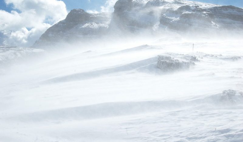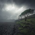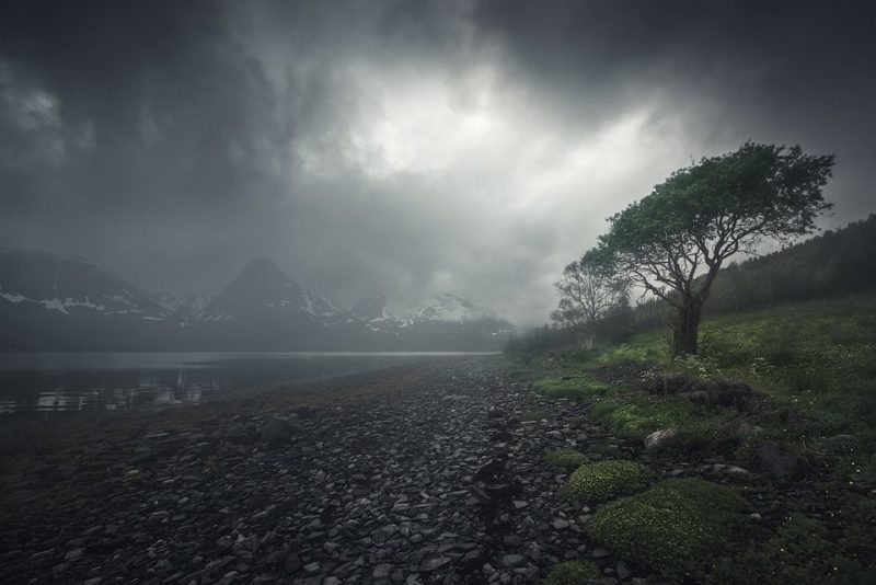
We study Earth’s history by studying the record of past events that is preserved in the rocks. Image via Guy Ottewell.
Re-printed with permission from Guy Ottewell’s blog; click here to visit him.
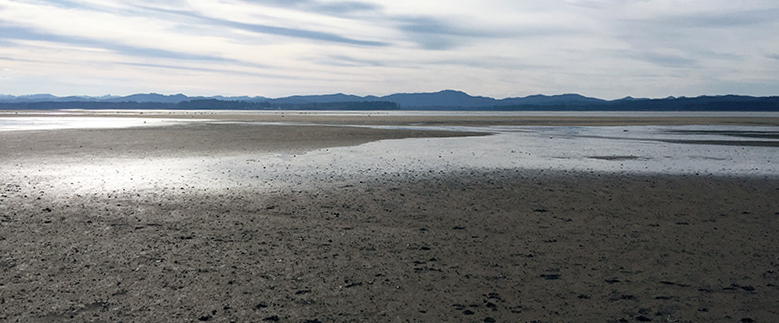
We are now on what is called the Jurassic Coast, on the English Channel coast of southern England. It was given this title after it became a UNESCO World Heritage Site in 2001. Jurassic is the name of just one of a group of three geological layers, but it’s the one more popularly known because of the 1993 film Jurassic Park, so is good for tourism.
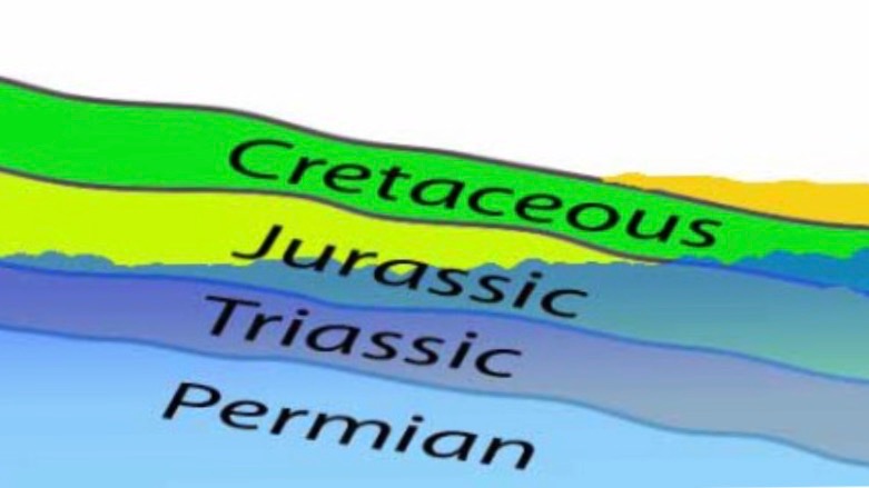
The three layers – Triassic, Jurassic, and Cretaceous – underlie much of England, and became tilted so that they slope gently down toward the east. They are collectively called the Mesozoic (which means middle life); the era in which they were laid down is also known as the Age of Dinosaurs. It lasted from about 250 million to about 65 million years ago. The three layers outcrop along this coast in cliffs, from which fossils are loosened by tides and landslips, so Lyme Regis, in the middle of the Jurassic Coast, is a mecca for geologists.
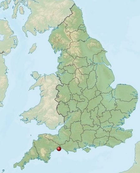
Location of the Jurassic Coast in England, via Wikipedia.
What happened 250 million years ago to begin the Mesozoic? The time period is known as the Permian-Triassic extinction, when 70 percent of all life on land, and 90 percent of all life in the oceans, was wiped out. The causes aren’t known precisely, but massive volcanic eruptions in what is now Siberia were involved. Carbon dioxide was forced into the oceans, and oxygen forced out. Marine life asphyxiated.
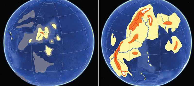
Life had previously been diverse. It had radiated in the Cambrian explosion – an event some 541 million years ago, when most major animal phyla appeared in the fossil record – into all the lineages that still exist and many that do not.
Perhaps, if the great extinction hadn’t happened, we would be 250 million years more advanced than we now are.
Life began thriving and diversifying again, through the Triassic, Jurassic, and Cretaceous periods. Then about 65 million years ago came another extinction, called the Cretaceous-Paleogene. It was more scary than Jurassic Park but maybe not quite as drastic as the earlier event: it extinguished three quarters of species. It is thought to have been caused by an asteroid that hit the Yucatán, and is more popularly known, because it killed all dinosaurs except the birds.
We are living spatially above the traces of those global extinctions, and, in time, within another, between the recent geological period called the Holocene and what is coming to be called a new one, the Anthropocene. It began with agriculture, and has been accelerating since the industrial revolution. Carbon dioxide is again being forced into the oceans, so that corals are dying.
Of the world’s mammals, 36 percent, by mass, are now of one species, the human. I’ve read that 60 percent are livestock grown for human use (cattle, sheep, pigs). Wild mammals (everything from whales to elephants to lions to lemurs to mice) are reduced to 4 percent. Of birds, 70 percent by mass are livestock (poultry); wild birds are down to 30 percent. These are among the findings of the first thorough assessment of the world’s biomass, reported on May 21, 2018 in the Proceedings of the National Academy of Sciences of the U.S.A.
No need to repeat the statistics of the declines of fish, amphibians, bees, of which you’ve doubtless read. A recent shock was the decimation in European countries, probably extrapolable to others, of all flying insects, on which the higher food chain depends.
I’m not sure how the ongoing extinction event compares with the Permian-Triassic one in speed and scale. But it shouldn’t be as bad. Its cause is not a blind volcanic force but a cognitive species, which will presumably understand and change its behavior before those percentages reach their worst.
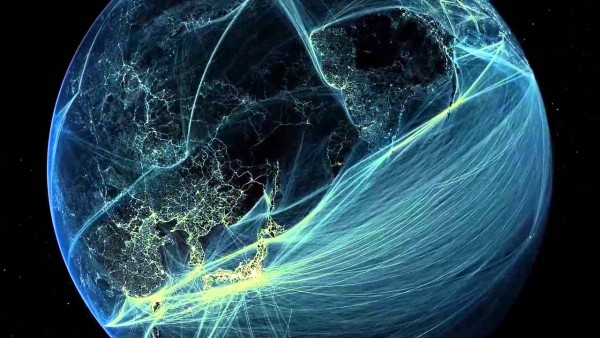
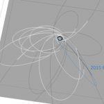
Image from a film called Welcome to the Anthropocene, commissioned by the Planet Under Pressure conference, London, March, 2012.
Bottom line: There have been multiple mass extinctions in Earth’s history. Signs point to our living in the midst of one now?
Source: The biomass distribution on Earth
Read more: The Anthropocene has begun
Watch: The Jurassic Coast, a 5-minute film below by Tim Britton
from EarthSky https://ift.tt/2IXlNDR
We study Earth’s history by studying the record of past events that is preserved in the rocks. Image via Guy Ottewell.
Re-printed with permission from Guy Ottewell’s blog; click here to visit him.
We are now on what is called the Jurassic Coast, on the English Channel coast of southern England. It was given this title after it became a UNESCO World Heritage Site in 2001. Jurassic is the name of just one of a group of three geological layers, but it’s the one more popularly known because of the 1993 film Jurassic Park, so is good for tourism.
The three layers – Triassic, Jurassic, and Cretaceous – underlie much of England, and became tilted so that they slope gently down toward the east. They are collectively called the Mesozoic (which means middle life); the era in which they were laid down is also known as the Age of Dinosaurs. It lasted from about 250 million to about 65 million years ago. The three layers outcrop along this coast in cliffs, from which fossils are loosened by tides and landslips, so Lyme Regis, in the middle of the Jurassic Coast, is a mecca for geologists.
Location of the Jurassic Coast in England, via Wikipedia.
What happened 250 million years ago to begin the Mesozoic? The time period is known as the Permian-Triassic extinction, when 70 percent of all life on land, and 90 percent of all life in the oceans, was wiped out. The causes aren’t known precisely, but massive volcanic eruptions in what is now Siberia were involved. Carbon dioxide was forced into the oceans, and oxygen forced out. Marine life asphyxiated.
Life had previously been diverse. It had radiated in the Cambrian explosion – an event some 541 million years ago, when most major animal phyla appeared in the fossil record – into all the lineages that still exist and many that do not.
Perhaps, if the great extinction hadn’t happened, we would be 250 million years more advanced than we now are.
Life began thriving and diversifying again, through the Triassic, Jurassic, and Cretaceous periods. Then about 65 million years ago came another extinction, called the Cretaceous-Paleogene. It was more scary than Jurassic Park but maybe not quite as drastic as the earlier event: it extinguished three quarters of species. It is thought to have been caused by an asteroid that hit the Yucatán, and is more popularly known, because it killed all dinosaurs except the birds.
We are living spatially above the traces of those global extinctions, and, in time, within another, between the recent geological period called the Holocene and what is coming to be called a new one, the Anthropocene. It began with agriculture, and has been accelerating since the industrial revolution. Carbon dioxide is again being forced into the oceans, so that corals are dying.
Of the world’s mammals, 36 percent, by mass, are now of one species, the human. I’ve read that 60 percent are livestock grown for human use (cattle, sheep, pigs). Wild mammals (everything from whales to elephants to lions to lemurs to mice) are reduced to 4 percent. Of birds, 70 percent by mass are livestock (poultry); wild birds are down to 30 percent. These are among the findings of the first thorough assessment of the world’s biomass, reported on May 21, 2018 in the Proceedings of the National Academy of Sciences of the U.S.A.
No need to repeat the statistics of the declines of fish, amphibians, bees, of which you’ve doubtless read. A recent shock was the decimation in European countries, probably extrapolable to others, of all flying insects, on which the higher food chain depends.
I’m not sure how the ongoing extinction event compares with the Permian-Triassic one in speed and scale. But it shouldn’t be as bad. Its cause is not a blind volcanic force but a cognitive species, which will presumably understand and change its behavior before those percentages reach their worst.
Image from a film called Welcome to the Anthropocene, commissioned by the Planet Under Pressure conference, London, March, 2012.
Bottom line: There have been multiple mass extinctions in Earth’s history. Signs point to our living in the midst of one now?
Source: The biomass distribution on Earth
Read more: The Anthropocene has begun
Watch: The Jurassic Coast, a 5-minute film below by Tim Britton
from EarthSky https://ift.tt/2IXlNDR