After publishing my experiences talking to science 'dismissives' (or 'skeptics', or whatever you'd like to call them) and then participating in the excellent Denial101x course, I was invited to join the volunteer team at SkepticalScience last year.
But before all that, one of the dismissives drew my attention to a climate science paradox:
- Scientists agree that the greenhouse effect is approximately logarithmic — which means that as we add more CO2 to the atmosphere, the effect of extra CO2 decreases.
- However, the IPCC projects that if we don't take steps to reduce our emissions, global warming won't just get worse, it will speed up:
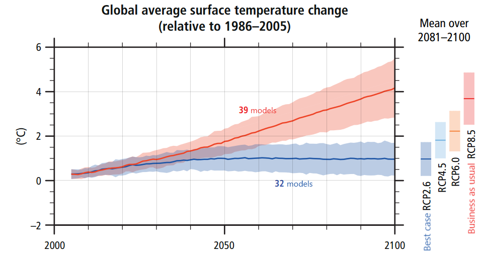
Figure 1: From IPCC AR5 synthesis report, page 11
How could both facts be true, I wondered? At the time I turned to "Ask A Climate Scientist" on Facebook and got a response from Steve Sherwood, an atmospheric scientist and one of the hundreds of IPCC report authors. I thought my first post here at SkS would be a good opportunity to share what I learned.
So what is this "logarithmic effect" exactly? It looks like this:
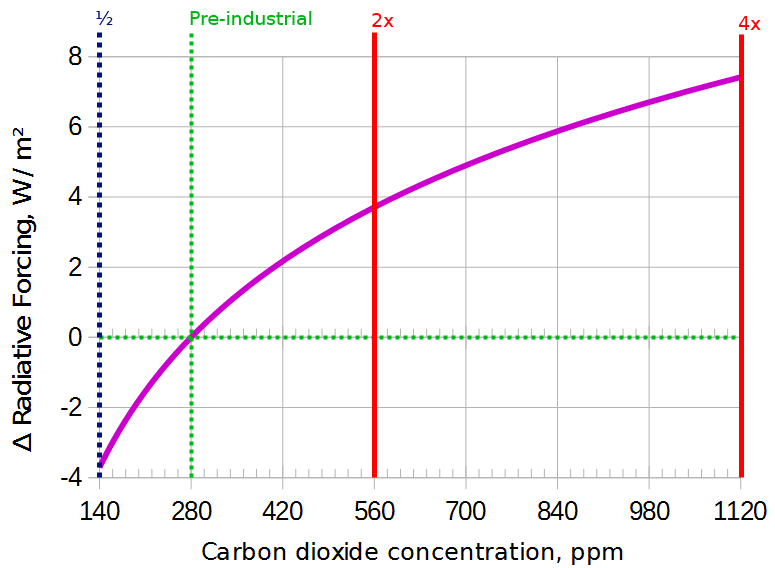
Figure 2: The surface receives about 3.7 W/m2 more energy each time CO2 is doubled.
In the last million years, CO2 levels have cycled between about 180 and 280 ppm during cycles about 100,000 years long. Because this happened in the steep part of the curve, a change of only 100 ppm (together with the Milankovich cycles) was enough to move the world in and out of the ice ages. Even though humans have increased the CO2 concentration by 130 ppm already, this extra 130 ppm has a smaller effect than the 100 ppm that was added naturally before.
But let's zoom in on the part that we actually care about: the modern era.
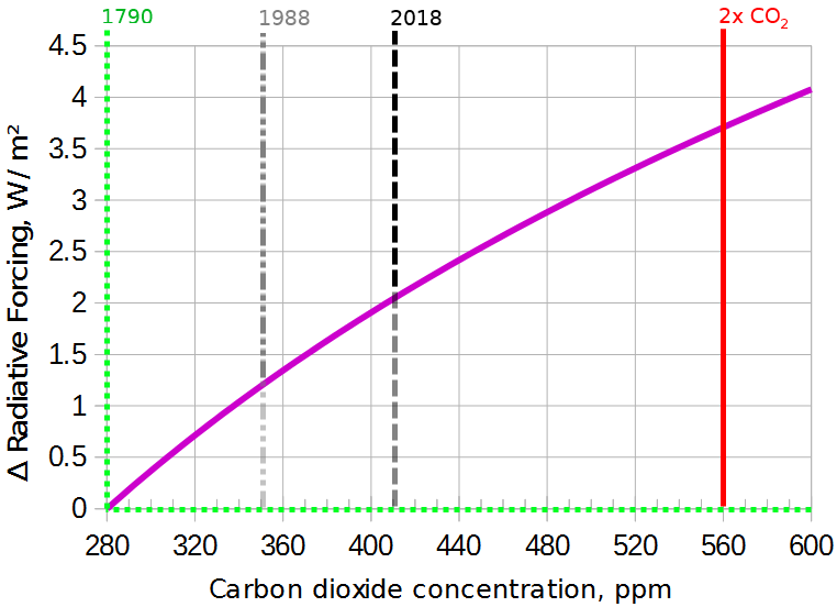
Figure 3
After zooming in, the logarithm doesn't make such a big difference: it's not far from a straight line. 560ppm will probably take us well beyond the Paris target of 1.5°C, so the 280-560 range is key; we would be unwise to let our civilization go beyond 560.
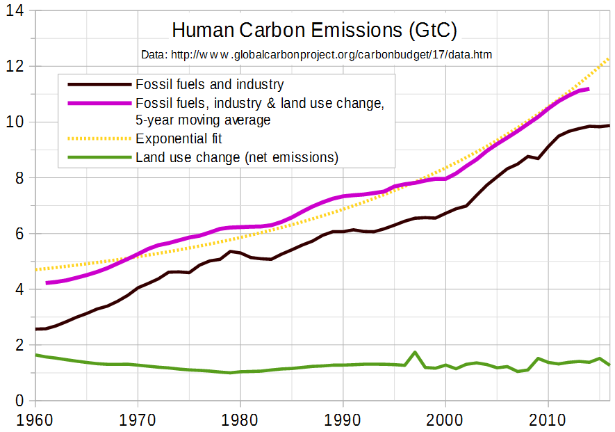
But human CO2 emissions are increasing exponentially—fast enough that when we plot atmospheric CO2 with a logarithmic scale, it still curves up, even over the last 30 years:
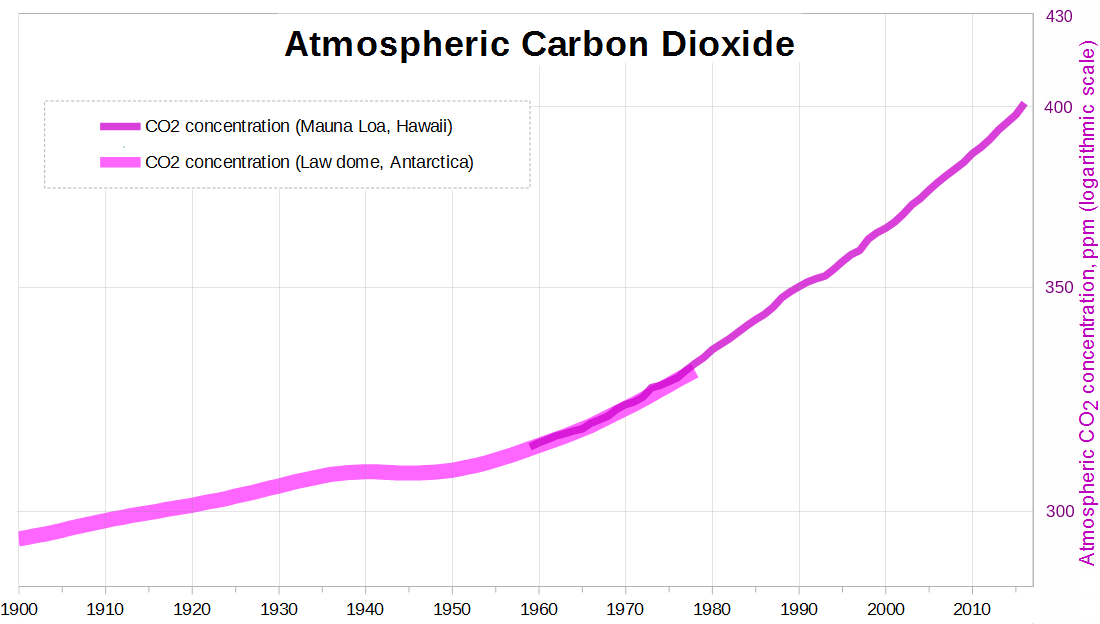
Figure 4
Exponential growth appears as a straight line on a logarithmic chart; an upward curve means, in some sense, faster than exponential growth.1 So if human emissions keep increasing as they have, it makes perfect sense that global warming would speed up.
"But wait," I hear you think, "surely it won't increase exponentially forever?" You're right, of course, it won't, but it could continue for awhile, and in total there are four factors that could work together to speed up warming:
- Rapid economic development
- Past emissions
- Carbon sink saturation
- Committed warming
1. The developing world is developing fast.
The late Hans Rosling explains this very well in his talk, "How Not to be Ignorant about the World". Poverty is decreasing faster than ever—which, I would think, means more power plants being built than ever before. Right now, about 1600 of those new power plants will burn coal. And as long as most of the world has a standard of living well below China's, there is plenty of room for growth to continue and perhaps even accelerate.
2. Past emissions (CO2 is cumulative)
Once we add CO2 to the atmosphere, we face the law of conservation of matter: it won't go away unless something removes it.
This is related to another paradox you might have heard: methane produces a much stronger greenhouse effect than CO2, yet scientists are less worried about it. Why? For one thing, it has a much lower concentration in the atmosphere, but what's really important here is that it has a short lifetime of only about 12 years before it is destroyed in the methane cycle. That makes the methane problem much less serious, as we expect nature will clean up the mess when we eventually reduce our methane output.
Carbon dioxide doesn't go away so easily. Here's a graph from Joos et al. (2013) estimating how slowly a large "pulse" (sudden addition) of CO2 would leave the atmosphere:
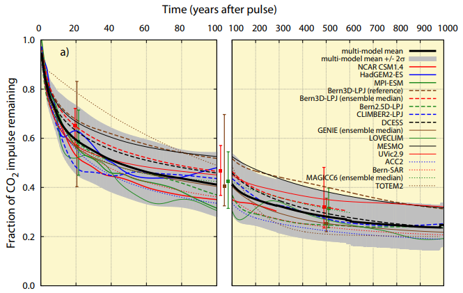
Figure 5
The black line is an average of many other studies and models. At first, the ocean and land absorb it "quickly", so about half of it is gone after "only" 50 years, locked up in seawater and plants. But the next 25% takes a full 950 years to go away! After 1000 years, the ocean has absorbed 59% (contributing to ocean acidification) and the land 16%, leaving 25% behind.
CO2 accumulation itself can't make global warming speed up, but what it does is prevent it from stopping by ensuring that the greenhouse forcing keeps going up. If you look at a graph of human emissions instead of atmospheric concentration, it's only roughly exponential. Human emissions temporarily stalled in the early 80s and early 90s, but since CO2 accumulates, the atmospheric curve just kept going up unabated.
3. Carbon sinks can saturate
Right now, carbon sinks (oceans, plants, and others) are removing about 2.4ppm of CO2 from the atmosphere each year, while we're adding about 5.2ppm, for a net increase of 2.5ppm per year.2
Figure 6: Where our emissions go (source)
While nature removes about half of our carbon emissions each year now, don't assume our good fortune will last. According to Jones et. al., 2013, there is disagreement between various climate models about the details, but on average, under the business-as-usual scenario known as RCP 8.5, the land is projected to absorb less CO2 as time goes on, and the fraction of our emissions absorbed by oceans will decrease too (even if the absolute absorption rate increases). In other words, just because we emit more doesn't guarantee nature absorbs more; sooner or later, CO2 will accumulate faster in the atmosphere. (On average about 2/3 of new emissions will stay in the atmosphere this century under RCP 8.5, where last century it was less than half.)
Basically, the oceans can absorb CO2 at first; increasing the CO2 in the air will always make oceans absorb more. However, as the oceans warm up, carbon solubility decreases—warm water can't hold as much of it, and the only reason ocean absorption will continue after that is that oceans are enormous and take time to "fill up", as the carbon spreads deeper and deeper. Given enough time, oceans would "saturate" and become unable to absorb more. Similarly, CO2 enhances plant growth to some extent, but growth is eventually balanced out by plant decomposition (which releases CO2), and the long-term effects of climate change won't necessarily be good for plants.
CO2 will eventually be removed permanently through a process called weathering—but this will take thousands of years.
4. Committed warming
Earth's climate system has feedback loops that magnify the warming effect of CO2. For example, as the arctic ice melts, it exposes ocean. The ocean is much darker than the ice, so more sunlight is absorbed instead of being reflected back to space. This enhances the arctic warming effect. This effect is time-delayed, since it takes many years for the arctic ocean to warm up (which in turn causes the ice to melt more quickly in the future, which in turn helps the ocean to heat up even more.)
"Committed warming" refers to future warming effects that would still happen even if CO2 levels stop increasing. A large source of delayed warming worldwide is the oceans, which, as you can see here, have not kept up with the warming of the land:
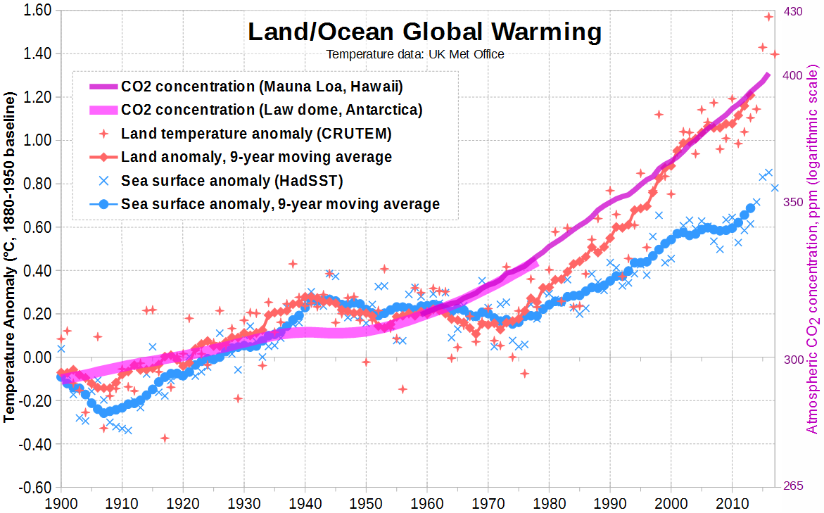
Figure 7
As our massive oceans slowly heat up, they will not only increase the global average surface temperature, but they will also warm up the land further, especially near the ocean where ocean temperature strongly affects the land.3
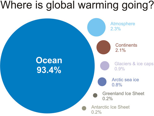
Figure 8 based on IPCC AR4 5.2.2.3
Due to this delayed warming, climate scientists have separate short-term and long-term estimates of global warming:

Figure 9: Warming from various CO2 levels based on a typical TCR estimate of 1.8°C and the most commonly-cited estimate of ECS, 3°C. Various scientific groups have produced a range of TCR and ECS estimates; the precise concentration of CO2 that corresponds to 1.5°C is unknown (the bars marked "Paris target" are drawn wide to represent the uncertainty, but are not scientifically accurate error bars). And of course, this graph is just a first-order approximation. The real climate will be warmed further by other greenhouse gases, especially methane, and the real climate has additional variability and unpredictability, as do all computer models of it.
As you can see, in the short term there is technically still time to fulfill the Paris agreement and keep global warming under 1.5°C—but this graph ignores methane, which moves the target closer. Unfortunately it is considered highly unlikely that we'll be able to stop at our 1.5°C goal.
The long term outlook is even worse: we've already passed 1.5.
The good news is that reaching the long-term "equilibrium" climate will take hundreds of years, giving us time to, hopefully, reverse course and avoid a lot of that committed warming. But it's very likely—especially after we pass 1.5°C—that humanity will someday need to figure out how to remove CO2 from the atmosphere on a large scale.
In summary:
Although CO2 has less effect at higher CO2 concentrations, this "logarithmic effect" will be overpowered by these 4 factors if we don't switch to clean energy quickly:
- Exponential growth of energy use
- Past CO2 emissions that nature has not yet absorbed
- Carbon sink saturation
- Committed warming
What if we manage to stop increasing our emissions? This related article indicates that if emissions hold steady, global warming will still continue upward linearly.
Good news though: the price of solar panels has passed an important milestone. Around the equator where sunlight is strongest, unsubsidized solar power plants have dropped below the price of coal. Hooray for Swanson's law! I also like to point out that a new kind of safe and cheap nuclear reactor will—if the public supports it—begin production in the 2020s. And on a graph of human CO2 emissions you can see emissions have stalled. Is this temporary, like it was in the early 80s and 90s, or are we finally at a turning point? Perhaps, but the IEA forecast still includes new fossil fuel plants in the coming years.
Footnotes
1 This may sound more dramatic than it is; the human emission increase has been exponential, not faster than exponential, so the upward curvature is caused by something else. I believe it's because we're in a transition region between roughly constant CO2 of the past (280 ppm) and the new pattern of exponentially increasing CO2. Inside the transition region, an upward curve is expected.
2 Note: due to uncertainties, the numbers don't add up perfectly (2.4+2.5≠5.2). These numbers are based on the average of the last 5 years of Global Carbon Budget data, i.e. 9.8 GtC emitted by humans per year, 1.39 GtC added via land-use change, 2.5 GtC removed by oceans and 2.63 GtC removed by land. These numbers are estimates, and the observed change is 2.51 ppm (5.32 GtC) per year, which is 0.33 ppm (0.71 GtC) different than expected. Data sources and uncertainty levels are listed here. The conversion factor is 2.13 GtC/ppm.
3 There is some good news: climate models say the oceans will never warm up as much as the land does. See Sutton et al. 2007 for details.
P.S. Why does CO2 have a logarithmic effect? It's complicated; see Myhre et al. (2008) or Huang & Shahabadi (2014) for technical details.
from Skeptical Science https://ift.tt/2Gi890H
After publishing my experiences talking to science 'dismissives' (or 'skeptics', or whatever you'd like to call them) and then participating in the excellent Denial101x course, I was invited to join the volunteer team at SkepticalScience last year.
But before all that, one of the dismissives drew my attention to a climate science paradox:
- Scientists agree that the greenhouse effect is approximately logarithmic — which means that as we add more CO2 to the atmosphere, the effect of extra CO2 decreases.
- However, the IPCC projects that if we don't take steps to reduce our emissions, global warming won't just get worse, it will speed up:
Figure 1: From IPCC AR5 synthesis report, page 11
How could both facts be true, I wondered? At the time I turned to "Ask A Climate Scientist" on Facebook and got a response from Steve Sherwood, an atmospheric scientist and one of the hundreds of IPCC report authors. I thought my first post here at SkS would be a good opportunity to share what I learned.
So what is this "logarithmic effect" exactly? It looks like this:
Figure 2: The surface receives about 3.7 W/m2 more energy each time CO2 is doubled.
In the last million years, CO2 levels have cycled between about 180 and 280 ppm during cycles about 100,000 years long. Because this happened in the steep part of the curve, a change of only 100 ppm (together with the Milankovich cycles) was enough to move the world in and out of the ice ages. Even though humans have increased the CO2 concentration by 130 ppm already, this extra 130 ppm has a smaller effect than the 100 ppm that was added naturally before.
But let's zoom in on the part that we actually care about: the modern era.
Figure 3
After zooming in, the logarithm doesn't make such a big difference: it's not far from a straight line. 560ppm will probably take us well beyond the Paris target of 1.5°C, so the 280-560 range is key; we would be unwise to let our civilization go beyond 560.
But human CO2 emissions are increasing exponentially—fast enough that when we plot atmospheric CO2 with a logarithmic scale, it still curves up, even over the last 30 years:
Figure 4
Exponential growth appears as a straight line on a logarithmic chart; an upward curve means, in some sense, faster than exponential growth.1 So if human emissions keep increasing as they have, it makes perfect sense that global warming would speed up.
"But wait," I hear you think, "surely it won't increase exponentially forever?" You're right, of course, it won't, but it could continue for awhile, and in total there are four factors that could work together to speed up warming:
- Rapid economic development
- Past emissions
- Carbon sink saturation
- Committed warming
1. The developing world is developing fast.
The late Hans Rosling explains this very well in his talk, "How Not to be Ignorant about the World". Poverty is decreasing faster than ever—which, I would think, means more power plants being built than ever before. Right now, about 1600 of those new power plants will burn coal. And as long as most of the world has a standard of living well below China's, there is plenty of room for growth to continue and perhaps even accelerate.
2. Past emissions (CO2 is cumulative)
Once we add CO2 to the atmosphere, we face the law of conservation of matter: it won't go away unless something removes it.
This is related to another paradox you might have heard: methane produces a much stronger greenhouse effect than CO2, yet scientists are less worried about it. Why? For one thing, it has a much lower concentration in the atmosphere, but what's really important here is that it has a short lifetime of only about 12 years before it is destroyed in the methane cycle. That makes the methane problem much less serious, as we expect nature will clean up the mess when we eventually reduce our methane output.
Carbon dioxide doesn't go away so easily. Here's a graph from Joos et al. (2013) estimating how slowly a large "pulse" (sudden addition) of CO2 would leave the atmosphere:
Figure 5
The black line is an average of many other studies and models. At first, the ocean and land absorb it "quickly", so about half of it is gone after "only" 50 years, locked up in seawater and plants. But the next 25% takes a full 950 years to go away! After 1000 years, the ocean has absorbed 59% (contributing to ocean acidification) and the land 16%, leaving 25% behind.
CO2 accumulation itself can't make global warming speed up, but what it does is prevent it from stopping by ensuring that the greenhouse forcing keeps going up. If you look at a graph of human emissions instead of atmospheric concentration, it's only roughly exponential. Human emissions temporarily stalled in the early 80s and early 90s, but since CO2 accumulates, the atmospheric curve just kept going up unabated.
3. Carbon sinks can saturate
Right now, carbon sinks (oceans, plants, and others) are removing about 2.4ppm of CO2 from the atmosphere each year, while we're adding about 5.2ppm, for a net increase of 2.5ppm per year.2
Figure 6: Where our emissions go (source)
While nature removes about half of our carbon emissions each year now, don't assume our good fortune will last. According to Jones et. al., 2013, there is disagreement between various climate models about the details, but on average, under the business-as-usual scenario known as RCP 8.5, the land is projected to absorb less CO2 as time goes on, and the fraction of our emissions absorbed by oceans will decrease too (even if the absolute absorption rate increases). In other words, just because we emit more doesn't guarantee nature absorbs more; sooner or later, CO2 will accumulate faster in the atmosphere. (On average about 2/3 of new emissions will stay in the atmosphere this century under RCP 8.5, where last century it was less than half.)
Basically, the oceans can absorb CO2 at first; increasing the CO2 in the air will always make oceans absorb more. However, as the oceans warm up, carbon solubility decreases—warm water can't hold as much of it, and the only reason ocean absorption will continue after that is that oceans are enormous and take time to "fill up", as the carbon spreads deeper and deeper. Given enough time, oceans would "saturate" and become unable to absorb more. Similarly, CO2 enhances plant growth to some extent, but growth is eventually balanced out by plant decomposition (which releases CO2), and the long-term effects of climate change won't necessarily be good for plants.
CO2 will eventually be removed permanently through a process called weathering—but this will take thousands of years.
4. Committed warming
Earth's climate system has feedback loops that magnify the warming effect of CO2. For example, as the arctic ice melts, it exposes ocean. The ocean is much darker than the ice, so more sunlight is absorbed instead of being reflected back to space. This enhances the arctic warming effect. This effect is time-delayed, since it takes many years for the arctic ocean to warm up (which in turn causes the ice to melt more quickly in the future, which in turn helps the ocean to heat up even more.)
"Committed warming" refers to future warming effects that would still happen even if CO2 levels stop increasing. A large source of delayed warming worldwide is the oceans, which, as you can see here, have not kept up with the warming of the land:
Figure 7
As our massive oceans slowly heat up, they will not only increase the global average surface temperature, but they will also warm up the land further, especially near the ocean where ocean temperature strongly affects the land.3
Figure 8 based on IPCC AR4 5.2.2.3
Due to this delayed warming, climate scientists have separate short-term and long-term estimates of global warming:
Figure 9: Warming from various CO2 levels based on a typical TCR estimate of 1.8°C and the most commonly-cited estimate of ECS, 3°C. Various scientific groups have produced a range of TCR and ECS estimates; the precise concentration of CO2 that corresponds to 1.5°C is unknown (the bars marked "Paris target" are drawn wide to represent the uncertainty, but are not scientifically accurate error bars). And of course, this graph is just a first-order approximation. The real climate will be warmed further by other greenhouse gases, especially methane, and the real climate has additional variability and unpredictability, as do all computer models of it.
As you can see, in the short term there is technically still time to fulfill the Paris agreement and keep global warming under 1.5°C—but this graph ignores methane, which moves the target closer. Unfortunately it is considered highly unlikely that we'll be able to stop at our 1.5°C goal.
The long term outlook is even worse: we've already passed 1.5.
The good news is that reaching the long-term "equilibrium" climate will take hundreds of years, giving us time to, hopefully, reverse course and avoid a lot of that committed warming. But it's very likely—especially after we pass 1.5°C—that humanity will someday need to figure out how to remove CO2 from the atmosphere on a large scale.
In summary:
Although CO2 has less effect at higher CO2 concentrations, this "logarithmic effect" will be overpowered by these 4 factors if we don't switch to clean energy quickly:
- Exponential growth of energy use
- Past CO2 emissions that nature has not yet absorbed
- Carbon sink saturation
- Committed warming
What if we manage to stop increasing our emissions? This related article indicates that if emissions hold steady, global warming will still continue upward linearly.
Good news though: the price of solar panels has passed an important milestone. Around the equator where sunlight is strongest, unsubsidized solar power plants have dropped below the price of coal. Hooray for Swanson's law! I also like to point out that a new kind of safe and cheap nuclear reactor will—if the public supports it—begin production in the 2020s. And on a graph of human CO2 emissions you can see emissions have stalled. Is this temporary, like it was in the early 80s and 90s, or are we finally at a turning point? Perhaps, but the IEA forecast still includes new fossil fuel plants in the coming years.
Footnotes
1 This may sound more dramatic than it is; the human emission increase has been exponential, not faster than exponential, so the upward curvature is caused by something else. I believe it's because we're in a transition region between roughly constant CO2 of the past (280 ppm) and the new pattern of exponentially increasing CO2. Inside the transition region, an upward curve is expected.
2 Note: due to uncertainties, the numbers don't add up perfectly (2.4+2.5≠5.2). These numbers are based on the average of the last 5 years of Global Carbon Budget data, i.e. 9.8 GtC emitted by humans per year, 1.39 GtC added via land-use change, 2.5 GtC removed by oceans and 2.63 GtC removed by land. These numbers are estimates, and the observed change is 2.51 ppm (5.32 GtC) per year, which is 0.33 ppm (0.71 GtC) different than expected. Data sources and uncertainty levels are listed here. The conversion factor is 2.13 GtC/ppm.
3 There is some good news: climate models say the oceans will never warm up as much as the land does. See Sutton et al. 2007 for details.
P.S. Why does CO2 have a logarithmic effect? It's complicated; see Myhre et al. (2008) or Huang & Shahabadi (2014) for technical details.
from Skeptical Science https://ift.tt/2Gi890H


