Close-up on a giant star

The different colors on the star’s surface correspond to varying temperatures. A star doesn’t have the same surface temperature throughout, and its surface provides our only clues to understand its internals. As temperatures rise and fall, the hotter, more fluid areas become brighter colors (such as white) and the cooler, more dense areas become darker colors (such as red). Image via ESO/Georgia State University.

An international team of astronomers has produced the first detailed image of the surface of a giant star – named Pi¹Gruis – that’s about 530 light-years from Earth in the constellation Grus (Latin for ‘crane’). It has about the same mass as our sun, but is 350 times larger and several thousand times as bright.

Pi¹Gruis is a red giant, a star in the last major phase of life, the researchers said, and resembles what the sun will become at the end of its life in five billion years.

The imaging reveals a nearly circular, dust-free atmosphere with complex areas of moving material, known as convection cells or granules, according to a study published December 20, 2017 in the journal Nature. According to a statement from the researchers:

Convection, the transfer of heat due to the bulk movement of molecules within gases and liquids, plays a major role in astrophysical processes, such as energy transport, pulsation and winds.

The researchers found that the surface of Pi¹Gruis has just a few convective cells, or granules, that are each about 74.5 million miles (120 million km) across — about a quarter of the star’s diameter. Just one of these granules would extend from the sun to beyond Venus.

By comparison, the sun’s surface contains about two million convective cells, with typical diameters of just 930 miles (1,500 km). The vast size differences in the convective cells of these two stars can be explained in part by their varying surface gravities, said the researchers. Pi¹Gruis is just 1.5 times the mass of the sun but much larger, resulting in a much lower surface gravity and just a few, extremely large, granules.

For the study, the team used the Precision Integrated-Optics Near-infrared Imaging ExpeRiment (PIONIER) instrument on the ESO’s Very Large Telescope Interferometer (VLTI) in Chile to observe the star. Researcher Fabien Baron is assistant professor in the Department of Physics and Astronomy at Georgia State University. Baron said in a statement:

This is the first time that we have such a giant star that is unambiguously imaged with that level of details. The reason is there’s a limit to the details we can see based on the size of the telescope used for the observations. For this paper, we used an interferometer. The light from several telescopes is combined to overcome the limit of each telescope, thus achieving a resolution equivalent to that of a much larger telescope.

Enjoying EarthSky so far? Sign up for our free daily newsletter today!

Bottom line: An international team of astronomers have created the first-ever detailed image of the surface of a giant star, 350 times larger than our sun.

Read more from Gerogia State University

from EarthSky http://ift.tt/2GtBuBM

The different colors on the star’s surface correspond to varying temperatures. A star doesn’t have the same surface temperature throughout, and its surface provides our only clues to understand its internals. As temperatures rise and fall, the hotter, more fluid areas become brighter colors (such as white) and the cooler, more dense areas become darker colors (such as red). Image via ESO/Georgia State University.

An international team of astronomers has produced the first detailed image of the surface of a giant star – named Pi¹Gruis – that’s about 530 light-years from Earth in the constellation Grus (Latin for ‘crane’). It has about the same mass as our sun, but is 350 times larger and several thousand times as bright.

Pi¹Gruis is a red giant, a star in the last major phase of life, the researchers said, and resembles what the sun will become at the end of its life in five billion years.

The imaging reveals a nearly circular, dust-free atmosphere with complex areas of moving material, known as convection cells or granules, according to a study published December 20, 2017 in the journal Nature. According to a statement from the researchers:

Convection, the transfer of heat due to the bulk movement of molecules within gases and liquids, plays a major role in astrophysical processes, such as energy transport, pulsation and winds.

The researchers found that the surface of Pi¹Gruis has just a few convective cells, or granules, that are each about 74.5 million miles (120 million km) across — about a quarter of the star’s diameter. Just one of these granules would extend from the sun to beyond Venus.

By comparison, the sun’s surface contains about two million convective cells, with typical diameters of just 930 miles (1,500 km). The vast size differences in the convective cells of these two stars can be explained in part by their varying surface gravities, said the researchers. Pi¹Gruis is just 1.5 times the mass of the sun but much larger, resulting in a much lower surface gravity and just a few, extremely large, granules.

For the study, the team used the Precision Integrated-Optics Near-infrared Imaging ExpeRiment (PIONIER) instrument on the ESO’s Very Large Telescope Interferometer (VLTI) in Chile to observe the star. Researcher Fabien Baron is assistant professor in the Department of Physics and Astronomy at Georgia State University. Baron said in a statement:

This is the first time that we have such a giant star that is unambiguously imaged with that level of details. The reason is there’s a limit to the details we can see based on the size of the telescope used for the observations. For this paper, we used an interferometer. The light from several telescopes is combined to overcome the limit of each telescope, thus achieving a resolution equivalent to that of a much larger telescope.

Enjoying EarthSky so far? Sign up for our free daily newsletter today!

Bottom line: An international team of astronomers have created the first-ever detailed image of the surface of a giant star, 350 times larger than our sun.

Read more from Gerogia State University

from EarthSky http://ift.tt/2GtBuBM

Double moon halo

Photo by nature photographer Josh Blash.

This photo – taken January 28, 2018 by Josh Blash in Hampton, New Hampshire – shows what’s called a halo around the moon. These sorts of halos are made by ice crystals in the upper air. In fact, there are two halos here, with the outer one being the common 22-degree halo, whose image we see several times each day in photos sent in by people around the world. The inner halo is more rare. We asked sky optics guru Les Cowley of the website Atmospheric Optics about the inner halo, and he said:

The inner ring looks like a diffuse 9-degree halo. This halo is formed by pyramidal ice crystals rather than the flat-ended prisms that make most halos.

The 9-degree halo is usually sharper. This one was probably generated by less-than-perfect crystals.

Pyramidal halos are fairly rare. Look out for them, but always shield the sun from both eyes. Mask it with a wall or tree.

See another photo of an intricate halo made by pyramidal ice crystals

Read more about 9-degree halo, and other halos made by pyramidal ice crystal, at Atmospheric Optics

Bottom line: Josh Blash captured this common 22-degree lunar halo, with a rarer 9-degree lunar halo inside it, on January 28, 2018.

from EarthSky http://ift.tt/2ElThtW

Photo by nature photographer Josh Blash.

This photo – taken January 28, 2018 by Josh Blash in Hampton, New Hampshire – shows what’s called a halo around the moon. These sorts of halos are made by ice crystals in the upper air. In fact, there are two halos here, with the outer one being the common 22-degree halo, whose image we see several times each day in photos sent in by people around the world. The inner halo is more rare. We asked sky optics guru Les Cowley of the website Atmospheric Optics about the inner halo, and he said:

The inner ring looks like a diffuse 9-degree halo. This halo is formed by pyramidal ice crystals rather than the flat-ended prisms that make most halos.

The 9-degree halo is usually sharper. This one was probably generated by less-than-perfect crystals.

Pyramidal halos are fairly rare. Look out for them, but always shield the sun from both eyes. Mask it with a wall or tree.

See another photo of an intricate halo made by pyramidal ice crystals

Read more about 9-degree halo, and other halos made by pyramidal ice crystal, at Atmospheric Optics

Bottom line: Josh Blash captured this common 22-degree lunar halo, with a rarer 9-degree lunar halo inside it, on January 28, 2018.

from EarthSky http://ift.tt/2ElThtW

Super Blue Moon eclipse on January 31

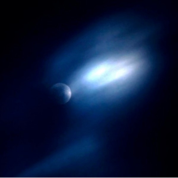
Total lunar eclipse photo, above, taken in 2004 by Fred Espenak

The Blue Moon – second of two full moons in one calendar month – will pass through the Earth’s shadow on January 31, 2018, to give us a total lunar eclipse. Totality, when the moon will be entirely inside the Earth’s dark umbral shadow, will last a bit more than one-and-a-quarter hours. The January 31 full moon is also the third in a series of three straight full moon supermoons – that is, super-close full moons. It’s the first of two Blue Moons in 2018. So it’s not just a total lunar eclipse, or a Blue Moon, or a supermoon. It’s all three … a super Blue Moon total eclipse!

Is it the first Blue Moon total eclipse in 150 years, as some social media memes are now claiming? It is … if you’re not considering the whole world, but only the Americas. More about that below.

How about supermoon total lunar eclipses? The last supermoon total lunar eclipse was in September 2015. And the last super Blue Moon total eclipse happened on December 30, 1982.

IMPORTANT. If you live in North America or the Hawaiian Islands, this lunar eclipse will be visible in your sky before sunrise on January 31.

On the other hand, if you live in the Middle East, Asia, Indonesia, Australia or New Zealand, this lunar eclipse will happen in the evening hours after sunset on January 31.

Follow the links below to learn eclipse times and more:

Eclipse times in Universal Time

Eclipse times for North American time zones

Eclipse calculators provide eclipse times for your sky

First Blue Moon total eclipse in 150 years? Well…

Who will see a partial lunar eclipse?

What causes a lunar eclipse?

January 31 is 1st of two Blue Moons in 2018

View larger. | Greatest eclipse happens at the same instant worldwide, but our clocks say different times. Chart by Fred Espenak. Click here for more details.

Eclipse times in Universal Time

Partial umbral eclipse begins: 11:48 Universal Time (UT)
Total eclipse begins: 12:52 UT
Greatest eclipse: 13:30 UT
Total eclipse ends: 14:08 UT
Partial umbral eclipse ends: 15:11 UT

How do I translate Universal Time to my time?

Eclipse times for North American time zones:

Eastern Standard Time (January 31, 2018)
Partial umbral eclipse begins: 6:48 a.m. EST
Moon sets before start of total eclipse

Central Standard Time (January 31, 2018)
Partial umbral eclipse begins: 5:48 a.m. CST
Total eclipse begins: 6:52 a.m. CST
Moon may set before totality ends

Mountain Standard Time (January 31, 2018)
Partial umbral eclipse begins: 4:48 a.m. MST
Total eclipse begins: 5:52 a.m. MST
Greatest eclipse: 6:30 a.m. MST
Total eclipse ends: 7:08 a.m. MST
Moon sets before end of partial umbral eclipse

Pacific Standard Time (January 31, 2018)
Partial umbral eclipse begins: 3:48 a.m. PST
Total eclipse begins: 4:52 a.m. PST
Greatest eclipse: 5:30 a.m. PST
Total eclipse ends: 6:08 a.m. PST
Partial umbral eclipse ends: 7:11 a.m. PST
Moon may set before end of partial umbral eclipse

Alaskan Standard Time (January 31, 2018)
Partial umbral eclipse begins: 2:48 a.m. AKST
Total eclipse begins: 3:52 a.m. AKST
Greatest eclipse: 4:30 a.m. AKST
Total eclipse ends: 5:08 a.m. AKST
Partial umbral eclipse ends: 6:11 a.m. AKST

Hawaii-Aleutian Standard Time (January 31, 2018)
Partial umbral eclipse begins: 1:48 a.m. HAST
Total eclipse begins: 2:52 a.m. HAST
Greatest eclipse: 3:30 a.m. HAST
Total eclipse ends: 4:08 a.m. HAST
Partial umbral eclipse ends: 5:11 a.m. HAST

Eclipse calculators provide eclipse times for your sky.

Remember … you have to be on the night side of Earth while the lunar eclipse is taking place to witness this great natural phenomenon. Of course, people around the globe want to know whether the eclipse is visible from their part of the world and at what time. To find out the local time of the greatest eclipse in your sky, click on this eclipse calculator and put in the name of a city near you. No time conversion is necessary for this eclipse calculator or the one below because the eclipse times are given in local time.

Eclipse computer via the US Naval Observatory

Animation of the 2018 January 31 total lunar eclipse. The moon travels eastward through the Earth’s penumbra (light outside shadow) and umbra (dark inner shadow). The yellow line depicts the ecliptic – Earth’s orbital plane. Although the moon, at least in part, spends a little over 3 1/3 hours within the umbra (dark shadow), it is only totally submerged in the umbra for about 1 1/4 hours.

In any umbral lunar eclipse, the moon always passes through Earth’s very light penumbral shadow before and after its journey through the dark umbral shadow.

First Blue Moon total eclipse in 150 years? Well… It depends on where you live. Yes, we’ve seen the social media memes going around suggesting this is the first Blue Moon total eclipse in 150 years. But the meme is true only for time zones in and around the Americas, not for the rest of the world. The last time that we had a Blue Moon total lunar eclipse – reckoning in world time (UTC, or GMT) – was December 30, 1982.

Full moon: 1982 December 1 at 00:21 UTC

Full moon: 1982 December 30 at 11:33 UTC (total lunar eclipse)

That wasn’t a Blue Moon eclipse for the Americas, however. For us, the full moon previous to the total lunar eclipse fell on November 30 – not December 1.

Before that, there was a Blue Moon total lunar eclipse for the world’s Eastern Hemisphere (Asia, Indonesia, Australia and New Zealand) on December 30, 1963.

Full Moon: 1963 November 30 at 23:54 UTC

Full Moon: 1963 December 30 at 11:04 UTC (total lunar eclipse)

Okay, now, finally we get to it. Before that, in late March 1866, there was a Blue Moon total lunar eclipse for North and South American time zones. But this full moon was not a supermoon.

Full Moon: 1866 March 1 at 11:52 UTC

Full Moon: 1866 March 31 at 4:32 UTC (total lunar eclipse)

By the way, the next Blue Moon total lunar eclipse will happen on December 31, 2028.

Source: Moon Phases by Fred Espenak

Who will see a partial lunar eclipse? A partial lunar eclipse precedes the total eclipse by a little over one hour, and follows totality for a little over one hour.

So, from start to finish, the moon takes 3 hours and 23 minutes to totally cross Earth’s dark umbral shadow. Eastern North America can see beginning stages of the partial umbral eclipse low in the west before sunrise January 31, whereas portions of the Middle East and far-eastern Europe can view the ending stages of the partial umbral eclipse low in the east after sunset January 31. South America, most of Europe and Africa won’t be able see this eclipse. See worldwide map below.

Incidentally, a very light penumbral eclipse comes before and after the dark (umbral) stage of the lunar eclipse. But this sort of eclipse is so faint that many people won’t even notice it. The penumbral eclipse would be more fun to watch from the moon, where it would be seen as a partial eclipse of the sun.

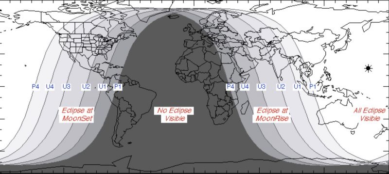
Worldwide map of the 2018 January 31 total lunar eclipse

View larger. Need help with the above map, courtesy of EclipseWise.com? Every place in white sees the whole eclipse from start to finish, whereas every place in black misses out entirely. Let EclipseWise.com by the eclipse master Fred Espenak walk you through the Key to Lunar Eclipse Figures. See less complicated map below.

Day and night sides of Earth at greatest total eclipse

Day and night sides of Earth at greatest eclipse (13:30 UT). The shadow line at left, running through North America, depicts sunrise (moonset). The shadow line at right, running through far-eastern Europe and far-western Asia depicts sunset (moonrise). Image credit: Earth View

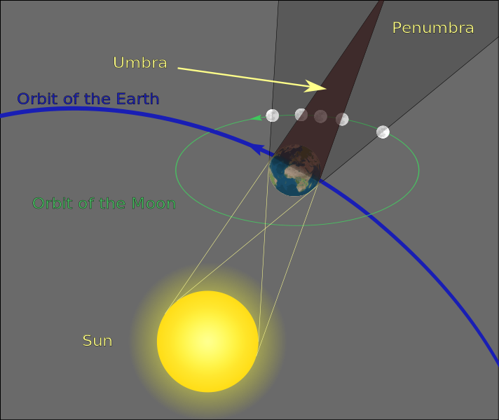
What causes a lunar eclipse? A lunar eclipse can only happen at full moon. Only then is it possible for the moon to be directly opposite the sun in our sky, and to pass into the Earth’s dark umbral shadow. Most of the time, however, the full moon eludes the Earth’s shadow by swinging to the north of it, or south of it. For instance, the last full moon on January 2, 2018, swung south of the Earth’s shadow. The next full moon – on March 2, 2018 – will swing north of the Earth’s shadow.

The moon’s orbital plane around Earth is actually inclined at 5 degrees to the ecliptic – Earth’s orbital plane around the sun. However, the moon’s orbit intersects the ecliptic at two points called nodes. It’s an ascending node where it crosses the Earth’s orbital plane going from south to north, and a descending node where it crosses the Earth’s orbital plane,going from north to south.

In short, a lunar eclipse happens when the full moon closely coincides with one of its nodes, and a solar eclipse happens when a new moon does likewise. It’s not a perfect alignment this time around, with the moon turning full about 5 hours before the moon crosses its ascending node. But that’s close enough for this full moon to stage a total lunar eclipse that lasts a touch more than one and 1/4 hours.

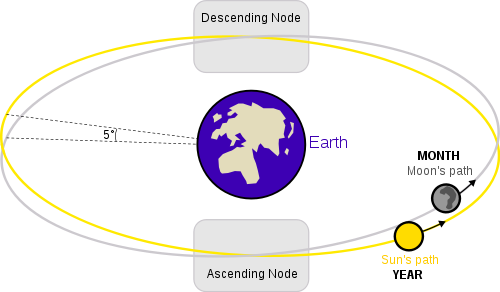
The yellow circle shows the sun’s apparent yearly path (the ecliptic) in front of the constellations of the Zodiac. The gray circle displays the monthly path of the moon in front of the zodiacal constellations. If a new moon or full moon aligns closely with one of the moon’s nodes, then an eclipse is in the works.

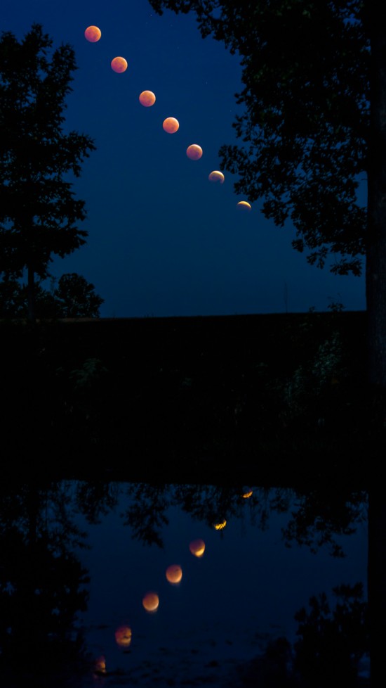
Time lapse of October 8, 2014, lunar eclipse as reflected in a pond in central Illinois, by Greg Lepper.

Bottom line: The super Blue Moon happens before sunrise on January 31, 2018, for North America and Hawaii. It happens after sunset on January 31 for the Middle East, Asia, Indonesia, Australia and New Zealand. Details here.

Need more details? Visit Fred Espenak’s page

EarthSky astronomy kits are perfect for beginners. Order today from the EarthSky store

Donate: Your support means the world to us

from EarthSky http://ift.tt/2BCJXjS

Total lunar eclipse photo, above, taken in 2004 by Fred Espenak

The Blue Moon – second of two full moons in one calendar month – will pass through the Earth’s shadow on January 31, 2018, to give us a total lunar eclipse. Totality, when the moon will be entirely inside the Earth’s dark umbral shadow, will last a bit more than one-and-a-quarter hours. The January 31 full moon is also the third in a series of three straight full moon supermoons – that is, super-close full moons. It’s the first of two Blue Moons in 2018. So it’s not just a total lunar eclipse, or a Blue Moon, or a supermoon. It’s all three … a super Blue Moon total eclipse!

Is it the first Blue Moon total eclipse in 150 years, as some social media memes are now claiming? It is … if you’re not considering the whole world, but only the Americas. More about that below.

How about supermoon total lunar eclipses? The last supermoon total lunar eclipse was in September 2015. And the last super Blue Moon total eclipse happened on December 30, 1982.

IMPORTANT. If you live in North America or the Hawaiian Islands, this lunar eclipse will be visible in your sky before sunrise on January 31.

On the other hand, if you live in the Middle East, Asia, Indonesia, Australia or New Zealand, this lunar eclipse will happen in the evening hours after sunset on January 31.

Follow the links below to learn eclipse times and more:

Eclipse times in Universal Time

Eclipse times for North American time zones

Eclipse calculators provide eclipse times for your sky

First Blue Moon total eclipse in 150 years? Well…

Who will see a partial lunar eclipse?

What causes a lunar eclipse?

January 31 is 1st of two Blue Moons in 2018

View larger. | Greatest eclipse happens at the same instant worldwide, but our clocks say different times. Chart by Fred Espenak. Click here for more details.

Eclipse times in Universal Time

Partial umbral eclipse begins: 11:48 Universal Time (UT)
Total eclipse begins: 12:52 UT
Greatest eclipse: 13:30 UT
Total eclipse ends: 14:08 UT
Partial umbral eclipse ends: 15:11 UT

How do I translate Universal Time to my time?

Eclipse times for North American time zones:

Eastern Standard Time (January 31, 2018)
Partial umbral eclipse begins: 6:48 a.m. EST
Moon sets before start of total eclipse

Central Standard Time (January 31, 2018)
Partial umbral eclipse begins: 5:48 a.m. CST
Total eclipse begins: 6:52 a.m. CST
Moon may set before totality ends

Mountain Standard Time (January 31, 2018)
Partial umbral eclipse begins: 4:48 a.m. MST
Total eclipse begins: 5:52 a.m. MST
Greatest eclipse: 6:30 a.m. MST
Total eclipse ends: 7:08 a.m. MST
Moon sets before end of partial umbral eclipse

Pacific Standard Time (January 31, 2018)
Partial umbral eclipse begins: 3:48 a.m. PST
Total eclipse begins: 4:52 a.m. PST
Greatest eclipse: 5:30 a.m. PST
Total eclipse ends: 6:08 a.m. PST
Partial umbral eclipse ends: 7:11 a.m. PST
Moon may set before end of partial umbral eclipse

Alaskan Standard Time (January 31, 2018)
Partial umbral eclipse begins: 2:48 a.m. AKST
Total eclipse begins: 3:52 a.m. AKST
Greatest eclipse: 4:30 a.m. AKST
Total eclipse ends: 5:08 a.m. AKST
Partial umbral eclipse ends: 6:11 a.m. AKST

Hawaii-Aleutian Standard Time (January 31, 2018)
Partial umbral eclipse begins: 1:48 a.m. HAST
Total eclipse begins: 2:52 a.m. HAST
Greatest eclipse: 3:30 a.m. HAST
Total eclipse ends: 4:08 a.m. HAST
Partial umbral eclipse ends: 5:11 a.m. HAST

Eclipse calculators provide eclipse times for your sky.

Remember … you have to be on the night side of Earth while the lunar eclipse is taking place to witness this great natural phenomenon. Of course, people around the globe want to know whether the eclipse is visible from their part of the world and at what time. To find out the local time of the greatest eclipse in your sky, click on this eclipse calculator and put in the name of a city near you. No time conversion is necessary for this eclipse calculator or the one below because the eclipse times are given in local time.

Eclipse computer via the US Naval Observatory

Animation of the 2018 January 31 total lunar eclipse. The moon travels eastward through the Earth’s penumbra (light outside shadow) and umbra (dark inner shadow). The yellow line depicts the ecliptic – Earth’s orbital plane. Although the moon, at least in part, spends a little over 3 1/3 hours within the umbra (dark shadow), it is only totally submerged in the umbra for about 1 1/4 hours.

In any umbral lunar eclipse, the moon always passes through Earth’s very light penumbral shadow before and after its journey through the dark umbral shadow.

First Blue Moon total eclipse in 150 years? Well… It depends on where you live. Yes, we’ve seen the social media memes going around suggesting this is the first Blue Moon total eclipse in 150 years. But the meme is true only for time zones in and around the Americas, not for the rest of the world. The last time that we had a Blue Moon total lunar eclipse – reckoning in world time (UTC, or GMT) – was December 30, 1982.

Full moon: 1982 December 1 at 00:21 UTC

Full moon: 1982 December 30 at 11:33 UTC (total lunar eclipse)

That wasn’t a Blue Moon eclipse for the Americas, however. For us, the full moon previous to the total lunar eclipse fell on November 30 – not December 1.

Before that, there was a Blue Moon total lunar eclipse for the world’s Eastern Hemisphere (Asia, Indonesia, Australia and New Zealand) on December 30, 1963.

Full Moon: 1963 November 30 at 23:54 UTC

Full Moon: 1963 December 30 at 11:04 UTC (total lunar eclipse)

Okay, now, finally we get to it. Before that, in late March 1866, there was a Blue Moon total lunar eclipse for North and South American time zones. But this full moon was not a supermoon.

Full Moon: 1866 March 1 at 11:52 UTC

Full Moon: 1866 March 31 at 4:32 UTC (total lunar eclipse)

By the way, the next Blue Moon total lunar eclipse will happen on December 31, 2028.

Source: Moon Phases by Fred Espenak

Who will see a partial lunar eclipse? A partial lunar eclipse precedes the total eclipse by a little over one hour, and follows totality for a little over one hour.

So, from start to finish, the moon takes 3 hours and 23 minutes to totally cross Earth’s dark umbral shadow. Eastern North America can see beginning stages of the partial umbral eclipse low in the west before sunrise January 31, whereas portions of the Middle East and far-eastern Europe can view the ending stages of the partial umbral eclipse low in the east after sunset January 31. South America, most of Europe and Africa won’t be able see this eclipse. See worldwide map below.

Incidentally, a very light penumbral eclipse comes before and after the dark (umbral) stage of the lunar eclipse. But this sort of eclipse is so faint that many people won’t even notice it. The penumbral eclipse would be more fun to watch from the moon, where it would be seen as a partial eclipse of the sun.

Worldwide map of the 2018 January 31 total lunar eclipse

View larger. Need help with the above map, courtesy of EclipseWise.com? Every place in white sees the whole eclipse from start to finish, whereas every place in black misses out entirely. Let EclipseWise.com by the eclipse master Fred Espenak walk you through the Key to Lunar Eclipse Figures. See less complicated map below.

Day and night sides of Earth at greatest total eclipse

Day and night sides of Earth at greatest eclipse (13:30 UT). The shadow line at left, running through North America, depicts sunrise (moonset). The shadow line at right, running through far-eastern Europe and far-western Asia depicts sunset (moonrise). Image credit: Earth View

What causes a lunar eclipse? A lunar eclipse can only happen at full moon. Only then is it possible for the moon to be directly opposite the sun in our sky, and to pass into the Earth’s dark umbral shadow. Most of the time, however, the full moon eludes the Earth’s shadow by swinging to the north of it, or south of it. For instance, the last full moon on January 2, 2018, swung south of the Earth’s shadow. The next full moon – on March 2, 2018 – will swing north of the Earth’s shadow.

The moon’s orbital plane around Earth is actually inclined at 5 degrees to the ecliptic – Earth’s orbital plane around the sun. However, the moon’s orbit intersects the ecliptic at two points called nodes. It’s an ascending node where it crosses the Earth’s orbital plane going from south to north, and a descending node where it crosses the Earth’s orbital plane,going from north to south.

In short, a lunar eclipse happens when the full moon closely coincides with one of its nodes, and a solar eclipse happens when a new moon does likewise. It’s not a perfect alignment this time around, with the moon turning full about 5 hours before the moon crosses its ascending node. But that’s close enough for this full moon to stage a total lunar eclipse that lasts a touch more than one and 1/4 hours.

The yellow circle shows the sun’s apparent yearly path (the ecliptic) in front of the constellations of the Zodiac. The gray circle displays the monthly path of the moon in front of the zodiacal constellations. If a new moon or full moon aligns closely with one of the moon’s nodes, then an eclipse is in the works.

Time lapse of October 8, 2014, lunar eclipse as reflected in a pond in central Illinois, by Greg Lepper.

Bottom line: The super Blue Moon happens before sunrise on January 31, 2018, for North America and Hawaii. It happens after sunset on January 31 for the Middle East, Asia, Indonesia, Australia and New Zealand. Details here.

Need more details? Visit Fred Espenak’s page

EarthSky astronomy kits are perfect for beginners. Order today from the EarthSky store

Donate: Your support means the world to us

from EarthSky http://ift.tt/2BCJXjS

Natural gas killed coal – now renewables and batteries are taking over

Over the past decade, coal has been increasingly replaced by cheaper, cleaner energy sources. US coal power production has dropped by 44% (866 terawatt-hours [TWh]). It’s been replaced by natural gas (up 45%, or 400 TWh), renewables (up 260%, or 200 TWh), and increased efficiency (the US uses 9%, or 371 TWh less electricity than a decade ago).

Evolution of the American power grid mix since 1960. Illustration: Carbon Brief

In other words, of the 866 TWh of lost coal power production, 46% was picked up by natural gas, 43% by increased efficiency, and 23% by renewables.

Natural gas is an unstable ‘bridge fuel’

While the shift away from coal is a positive development in slowing global warming by cutting carbon pollution, as Joe Romm has detailed for Climate Progress, research indicates that shifting to natural gas squanders most of those gains. For example, a 2014 study published in Environmental Research Letters found that when natural gas production is abundant, it crowds out both coal and renewables, resulting in little if any climate benefit. Part of the problem is significant methane leakage from natural gas drilling.

...abundant gas consistently results in both less coal and renewable energy use […] the quantity of methane leaked may ultimately determine whether the overall effect is to slightly reduce or actually increase cumulative emissions […] only climate policies bring about a significant reduction in future emissions from US electricity generation … We conclude that increased natural gas use for electricity will not substantially reduce US GHG emissions, and by delaying deployment of renewable energy technologies, may actually exacerbate the climate change problem in the long term.

Similarly, another 2014 study found that based on the latest estimates of methane leakage rates from natural gas drilling, replacing coal with natural gas provides little in the way of climate benefits. Though it’s been touted as a ‘bridge fuel’ to span the gap between coal and renewables, this research suggests natural gas isn’t significantly better than coal in terms of global warming effects, and thus may not be suitable for that purpose. The ‘bridge’ doesn’t appear to achieve its goal of steadily cutting our greenhouse gas emissions.

Renewables and batteries are starting to beat natural gas

California has been a national leader in clean energy. The state generates very little of its electricity from coal, but natural gas does supply more than a third of the state’s power. A quarter is generated by renewable sources like wind, solar, and geothermal plants, and another 10% comes from hydroelectric dams, on average. In 2017, renewables’ share increased by about 10%, displacing natural gas in the process.

In fact, California has an excess of natural gas power generation capabilities. Some natural gas plants are still essential for ensuring local grid reliability, but in many cases, clean energy resources like a combination of solar and storage can meet reliability needs.

In one recent example, the California Public Utilities Commission (CPUC) ordered Pacific Gas & Electric (PG&E) to procure energy storage (batteries) or “preferred resources” (renewables or increased efficiency and conservation) to meet a local reliability need in northern California. The order stemmed from an issue with a “peaker” natural gas plant (so-called because they switch on to meet high, peak electricity demand) operated in northern California. The operator (Calpine) was concerned that the plant was no longer economical, because it’s too infrequently used due largely to an abundance of renewable power. The contract they could receive for providing generation capacity to ensure grid reliability would not be high enough to cover costs to maintain the plant.

Instead of bidding their plant into the program overseen by the CPUC to ensure local reliability, Calpine went directly to the California Independent System Operator (CAISO) and requested a “reliability must-run resource” contract, which is a much higher payment than they would have received through the CPUC program. CPUC decided instead to require PG&E to fill the local reliability need with cleaner alternatives. The costs of renewable energy and battery storage have fallen so fast that the clean alternatives might now be cheaper than gas.

In another example, a proposed natural gas peaker plant in Oxnard, California was rejected when it was shown that the CAISO was using outdated battery storage costs from 2014. Given how quickly those prices have fallen, they could now potentially be competitive with natural gas peaker costs.

The redundancy and potential replacement of natural gas with cleaner alternatives extends far beyond these examples. Most electrical service providers in California are now required to develop integrated resource plans. These are electric grid planning documents that outline how the utilities will meet a number of California’s goals, including a 40% reduction in carbon pollution below 1990 levels and 50% electricity production from renewable sources by 2030. Meeting these goals will require replacing non-critical natural gas plants with renewable power.

And California is already installing battery storage systems at record pace. Tesla, AES Energy Storage, and Greensmith Energy Partners have all installed large battery storage facilities in California within the past year. Within 4 years, batteries are projected to be as cheap as natural gas “peakers,” and consistently cheaper with 10 years.

Click here to read the rest

from Skeptical Science http://ift.tt/2DQ5TfO

Over the past decade, coal has been increasingly replaced by cheaper, cleaner energy sources. US coal power production has dropped by 44% (866 terawatt-hours [TWh]). It’s been replaced by natural gas (up 45%, or 400 TWh), renewables (up 260%, or 200 TWh), and increased efficiency (the US uses 9%, or 371 TWh less electricity than a decade ago).

Evolution of the American power grid mix since 1960. Illustration: Carbon Brief

In other words, of the 866 TWh of lost coal power production, 46% was picked up by natural gas, 43% by increased efficiency, and 23% by renewables.

Natural gas is an unstable ‘bridge fuel’

While the shift away from coal is a positive development in slowing global warming by cutting carbon pollution, as Joe Romm has detailed for Climate Progress, research indicates that shifting to natural gas squanders most of those gains. For example, a 2014 study published in Environmental Research Letters found that when natural gas production is abundant, it crowds out both coal and renewables, resulting in little if any climate benefit. Part of the problem is significant methane leakage from natural gas drilling.

...abundant gas consistently results in both less coal and renewable energy use […] the quantity of methane leaked may ultimately determine whether the overall effect is to slightly reduce or actually increase cumulative emissions […] only climate policies bring about a significant reduction in future emissions from US electricity generation … We conclude that increased natural gas use for electricity will not substantially reduce US GHG emissions, and by delaying deployment of renewable energy technologies, may actually exacerbate the climate change problem in the long term.

Similarly, another 2014 study found that based on the latest estimates of methane leakage rates from natural gas drilling, replacing coal with natural gas provides little in the way of climate benefits. Though it’s been touted as a ‘bridge fuel’ to span the gap between coal and renewables, this research suggests natural gas isn’t significantly better than coal in terms of global warming effects, and thus may not be suitable for that purpose. The ‘bridge’ doesn’t appear to achieve its goal of steadily cutting our greenhouse gas emissions.

Renewables and batteries are starting to beat natural gas

California has been a national leader in clean energy. The state generates very little of its electricity from coal, but natural gas does supply more than a third of the state’s power. A quarter is generated by renewable sources like wind, solar, and geothermal plants, and another 10% comes from hydroelectric dams, on average. In 2017, renewables’ share increased by about 10%, displacing natural gas in the process.

In fact, California has an excess of natural gas power generation capabilities. Some natural gas plants are still essential for ensuring local grid reliability, but in many cases, clean energy resources like a combination of solar and storage can meet reliability needs.

In one recent example, the California Public Utilities Commission (CPUC) ordered Pacific Gas & Electric (PG&E) to procure energy storage (batteries) or “preferred resources” (renewables or increased efficiency and conservation) to meet a local reliability need in northern California. The order stemmed from an issue with a “peaker” natural gas plant (so-called because they switch on to meet high, peak electricity demand) operated in northern California. The operator (Calpine) was concerned that the plant was no longer economical, because it’s too infrequently used due largely to an abundance of renewable power. The contract they could receive for providing generation capacity to ensure grid reliability would not be high enough to cover costs to maintain the plant.

Instead of bidding their plant into the program overseen by the CPUC to ensure local reliability, Calpine went directly to the California Independent System Operator (CAISO) and requested a “reliability must-run resource” contract, which is a much higher payment than they would have received through the CPUC program. CPUC decided instead to require PG&E to fill the local reliability need with cleaner alternatives. The costs of renewable energy and battery storage have fallen so fast that the clean alternatives might now be cheaper than gas.

In another example, a proposed natural gas peaker plant in Oxnard, California was rejected when it was shown that the CAISO was using outdated battery storage costs from 2014. Given how quickly those prices have fallen, they could now potentially be competitive with natural gas peaker costs.

The redundancy and potential replacement of natural gas with cleaner alternatives extends far beyond these examples. Most electrical service providers in California are now required to develop integrated resource plans. These are electric grid planning documents that outline how the utilities will meet a number of California’s goals, including a 40% reduction in carbon pollution below 1990 levels and 50% electricity production from renewable sources by 2030. Meeting these goals will require replacing non-critical natural gas plants with renewable power.

And California is already installing battery storage systems at record pace. Tesla, AES Energy Storage, and Greensmith Energy Partners have all installed large battery storage facilities in California within the past year. Within 4 years, batteries are projected to be as cheap as natural gas “peakers,” and consistently cheaper with 10 years.

Click here to read the rest

from Skeptical Science http://ift.tt/2DQ5TfO

New method calculates equilibrium constant at the small scale

Mixing computational chemistry and theoretical math proved a winning formula for Emory chemist James Kindt (center), his graduate students (from left) Xiaokun Zhang and Lara Patel, and mathematics graduate students Olivia Beckwith and Robert Schneider.

By Carol Clark

Computational chemists and mathematicians have developed a new, fast method to calculate equilibrium constants using small-scale simulations — even when the Law of Mass Action does not apply.

The Journal of Chemical Theory and Computation published the resulting algorithm and software, which the researchers have named PEACH — an acronym for “partition-enabled analysis of cluster histograms” and a nod to the method’s development in Georgia at Emory University.

“Our method will allow computational chemists to make better predictions in simulations for a wide range of complex reactions — from how aerosols form in the atmosphere to how proteins come together to form amyloid filaments implicated in Alzheimer’s disease,” says James Kindt, an Emory professor of computational chemistry, whose lab led the work.

Previously it would require at least a week of computing time to do the calculations needed for such predictions. The PEACH system reduces that time to seconds by using tricks derived from number theory.

“Our tool can use a small set of data and then extrapolate the results to a large-system case to predict the big picture,” Kindt says.

“What made this project so fun and interesting is the cross-cultural aspects of it,” he adds. “Computational chemists and theoretical mathematicians use different languages and don’t often speak to one another. By working together we’ve happened onto something that appears to be on the frontiers of both fields.”

The research team includes Lara Patel and Xiaokun Zhang, who are both PhD students of chemistry in the Kindt lab, and number theorists Olivia Beckwith and Robert Schneider, Emory PhD candidates in the Department of Mathematics and Computer Science. Chris Weeden, as an Emory undergraduate, contributed to early stages of the work.

The equilibrium constant is a basic concept taught in first-year college chemistry. According to the Law of Mass Action, at a given temperature, no matter how much of a product and a reactant are mixed together — as long as they are at equilibrium — a certain ratio of product to reactant will equal the equilibrium constant.

“That equation always holds true at equilibrium for huge numbers of molecules,” Kindt says. “It doesn’t matter if it’s applied to a bucket of water or to a single drop of water — which consists of about a billion trillion molecules.”

At much smaller scales of around dozens of molecules, however, the Law of Mass Action breaks down and does not apply.

The Kindt lab uses computers to simulate the behavior of molecules, in particular how they self-assemble into clusters. Sodium octyl sulfate, or SOS, is one of the compounds the lab uses as an experimental model. SOS is a surfactant that can act as a detergent. It forms little clusters in water that can encapsulate oil and grease. Simulations of how SOS molecules come together can predict the distribution of sizes of clusters formed under different conditions, in order to improve the design of soaps and detergents, and to better understand biological processes such as how bile salts break down globules of fat during the digestive process.

In a key test of their model, the lab needed to make sure that the equilibrium for the assembly reaction of SOS molecules into clusters matched up with experiments.

“If we were to run simulations with huge numbers of molecules, we could count the clusters that were formed of each size, count the molecules that remained free of the clusters, and use this information to calculate the equilibrium constant for forming each size cluster,” Kindt says. “The challenge we faced was that it would take too long for the computers to perform simulations of sufficiently huge numbers of molecules to get this to work, and for the numbers of clustering molecules we could practically handle — around 50 — the Law of Mass Action wouldn’t work.”

Kindt decided to approach the problem by considering all the different ways the molecules in a reaction could group into clusters of different sizes in order to arrive at an average. After doing some reading, he realized that these different ways of molecules grouping were what number theorists call integer partitions.

A partition of a number is a sequence of positive integers that add up to that number. For instance, there are five partitions of the number 4 (4 = 3+1 = 2+2 = 2+1+1 = 1+1+1+1). The partition numbers grow at an incredible rate. The amount of partitions for the number 10 is 42. For the number 100, the partitions explode to more than 190,000,000.

That same explosion of possibilities occurs for the ways that molecules can cluster.

Lara Patel and Xiaokun Zhang worked on a “brute force” method to get a computer to run through every single way to combine 10 molecules of one type with 10 molecules of another type. The problem was it took one computer working a couple of days to do a single analysis. And the computational time needed if just a few more molecules were added to the analysis went up exponentially.

The computational chemists had hit a wall.

Kindt reached out to Ken Ono, a world-renowned number theorist in Emory's Mathematics and Computer Science Department, to see if any of his graduate students would be interested in taking a crack at the problem.

Olivia Beckwith and Robert Schneider jumped at the chance.

“The Kindt lab’s computer simulations show that classical theorems from partition theory actually occur in nature, even for small numbers of molecules,” Schneider says. “It was surprising and felt very cosmic to me to learn that number theory determines real-world events.”

“It was definitely unexpected,” adds Beckwith. “In theoretical math we tend to work in isolation from physical phenomena like the interaction of molecules.”

The chemists and mathematicians began meeting regularly to discuss the problem and to learn one another’s terminology. “I had to pull out my son’s high school chemistry book and spend a weekend reading through it,” Schneider says.

“It happened so organically,” Patel says of the process of blending their two specialties. “Olivia and Richard would write equations on the board and as soon as a formula made sense to me I’d start thinking in my head, ‘How can we code this so that we can apply it?’”

The two mathematicians suggested a strategy that could make the problem much easier to calculate, based on a theorem known as Faà di Bruno’s Formula.

“It was surprising,” Zhang says, “because it was an idea that never would have occurred to me. They helped us get unstuck and to find a way to push our research forward.”

“They helped us find a shortcut so that we didn’t have to generate all the partitions for ways that the molecules could clump together,” Kindt adds. “Their algorithm is a much more elegant and simple way to find the entire average overall.”

Patel and Zhang used this new algorithm to put together a piece of software to analyze data from the computer simulations. The resulting system, PEACH, speeds up calculations that previously took two hours to just one second. After demonstrating how PEACH simplifies simulations of SOS assemblages, the research team is moving on to simulate this process for a range of other molecules.

“We’re interested in describing how molecular structures dictate assembly in any type of scenario, such as the early stages of crystal formation,” Kindt says. “We’re also working on quantifying just where the Law of Mass Action breaks down. We could then refine the PEACH strategy to make it even more efficient.”

Related:
New theories reveal the nature of numbers

from eScienceCommons http://ift.tt/2nlGT5W

Mixing computational chemistry and theoretical math proved a winning formula for Emory chemist James Kindt (center), his graduate students (from left) Xiaokun Zhang and Lara Patel, and mathematics graduate students Olivia Beckwith and Robert Schneider.

By Carol Clark

Computational chemists and mathematicians have developed a new, fast method to calculate equilibrium constants using small-scale simulations — even when the Law of Mass Action does not apply.

The Journal of Chemical Theory and Computation published the resulting algorithm and software, which the researchers have named PEACH — an acronym for “partition-enabled analysis of cluster histograms” and a nod to the method’s development in Georgia at Emory University.

“Our method will allow computational chemists to make better predictions in simulations for a wide range of complex reactions — from how aerosols form in the atmosphere to how proteins come together to form amyloid filaments implicated in Alzheimer’s disease,” says James Kindt, an Emory professor of computational chemistry, whose lab led the work.

Previously it would require at least a week of computing time to do the calculations needed for such predictions. The PEACH system reduces that time to seconds by using tricks derived from number theory.

“Our tool can use a small set of data and then extrapolate the results to a large-system case to predict the big picture,” Kindt says.

“What made this project so fun and interesting is the cross-cultural aspects of it,” he adds. “Computational chemists and theoretical mathematicians use different languages and don’t often speak to one another. By working together we’ve happened onto something that appears to be on the frontiers of both fields.”

The research team includes Lara Patel and Xiaokun Zhang, who are both PhD students of chemistry in the Kindt lab, and number theorists Olivia Beckwith and Robert Schneider, Emory PhD candidates in the Department of Mathematics and Computer Science. Chris Weeden, as an Emory undergraduate, contributed to early stages of the work.

The equilibrium constant is a basic concept taught in first-year college chemistry. According to the Law of Mass Action, at a given temperature, no matter how much of a product and a reactant are mixed together — as long as they are at equilibrium — a certain ratio of product to reactant will equal the equilibrium constant.

“That equation always holds true at equilibrium for huge numbers of molecules,” Kindt says. “It doesn’t matter if it’s applied to a bucket of water or to a single drop of water — which consists of about a billion trillion molecules.”

At much smaller scales of around dozens of molecules, however, the Law of Mass Action breaks down and does not apply.

The Kindt lab uses computers to simulate the behavior of molecules, in particular how they self-assemble into clusters. Sodium octyl sulfate, or SOS, is one of the compounds the lab uses as an experimental model. SOS is a surfactant that can act as a detergent. It forms little clusters in water that can encapsulate oil and grease. Simulations of how SOS molecules come together can predict the distribution of sizes of clusters formed under different conditions, in order to improve the design of soaps and detergents, and to better understand biological processes such as how bile salts break down globules of fat during the digestive process.

In a key test of their model, the lab needed to make sure that the equilibrium for the assembly reaction of SOS molecules into clusters matched up with experiments.

“If we were to run simulations with huge numbers of molecules, we could count the clusters that were formed of each size, count the molecules that remained free of the clusters, and use this information to calculate the equilibrium constant for forming each size cluster,” Kindt says. “The challenge we faced was that it would take too long for the computers to perform simulations of sufficiently huge numbers of molecules to get this to work, and for the numbers of clustering molecules we could practically handle — around 50 — the Law of Mass Action wouldn’t work.”

Kindt decided to approach the problem by considering all the different ways the molecules in a reaction could group into clusters of different sizes in order to arrive at an average. After doing some reading, he realized that these different ways of molecules grouping were what number theorists call integer partitions.

A partition of a number is a sequence of positive integers that add up to that number. For instance, there are five partitions of the number 4 (4 = 3+1 = 2+2 = 2+1+1 = 1+1+1+1). The partition numbers grow at an incredible rate. The amount of partitions for the number 10 is 42. For the number 100, the partitions explode to more than 190,000,000.

That same explosion of possibilities occurs for the ways that molecules can cluster.

Lara Patel and Xiaokun Zhang worked on a “brute force” method to get a computer to run through every single way to combine 10 molecules of one type with 10 molecules of another type. The problem was it took one computer working a couple of days to do a single analysis. And the computational time needed if just a few more molecules were added to the analysis went up exponentially.

The computational chemists had hit a wall.

Kindt reached out to Ken Ono, a world-renowned number theorist in Emory's Mathematics and Computer Science Department, to see if any of his graduate students would be interested in taking a crack at the problem.

Olivia Beckwith and Robert Schneider jumped at the chance.

“The Kindt lab’s computer simulations show that classical theorems from partition theory actually occur in nature, even for small numbers of molecules,” Schneider says. “It was surprising and felt very cosmic to me to learn that number theory determines real-world events.”

“It was definitely unexpected,” adds Beckwith. “In theoretical math we tend to work in isolation from physical phenomena like the interaction of molecules.”

The chemists and mathematicians began meeting regularly to discuss the problem and to learn one another’s terminology. “I had to pull out my son’s high school chemistry book and spend a weekend reading through it,” Schneider says.

“It happened so organically,” Patel says of the process of blending their two specialties. “Olivia and Richard would write equations on the board and as soon as a formula made sense to me I’d start thinking in my head, ‘How can we code this so that we can apply it?’”

The two mathematicians suggested a strategy that could make the problem much easier to calculate, based on a theorem known as Faà di Bruno’s Formula.

“It was surprising,” Zhang says, “because it was an idea that never would have occurred to me. They helped us get unstuck and to find a way to push our research forward.”

“They helped us find a shortcut so that we didn’t have to generate all the partitions for ways that the molecules could clump together,” Kindt adds. “Their algorithm is a much more elegant and simple way to find the entire average overall.”

Patel and Zhang used this new algorithm to put together a piece of software to analyze data from the computer simulations. The resulting system, PEACH, speeds up calculations that previously took two hours to just one second. After demonstrating how PEACH simplifies simulations of SOS assemblages, the research team is moving on to simulate this process for a range of other molecules.

“We’re interested in describing how molecular structures dictate assembly in any type of scenario, such as the early stages of crystal formation,” Kindt says. “We’re also working on quantifying just where the Law of Mass Action breaks down. We could then refine the PEACH strategy to make it even more efficient.”

Related:
New theories reveal the nature of numbers

from eScienceCommons http://ift.tt/2nlGT5W

A Very Rare Super Blue Blood Moon Will Be Visible This Week… Here’s How to See it

A 'super blood blue moon' will be visible Jan. 31, with western North America, Asia, and the Middle East getting the best view. We'll tell you how to view it.

from http://ift.tt/2rROyxK

A 'super blood blue moon' will be visible Jan. 31, with western North America, Asia, and the Middle East getting the best view. We'll tell you how to view it.

from http://ift.tt/2rROyxK

What is a Blue Moon?

Most Blue Moons are not blue in color. This photo of a moon among fast-moving clouds was created using special filters. Image via EarthSky Facebook friend Jv Noriega.

In recent years, people have been using the name Blue Moon for the second of two full moons in a single calendar month. An older definition says a Blue Moon is the third of four full moons in a single season. Someday, you might see an actual blue-colored moon. The term once in a blue moon used to mean something rare. Now that the rules for naming Blue Moons include several different possibilities, Blue Moons are pretty common! The next Blue Moon (second full moon in one calendar month) will be January 31, 2018. Follow the links below to learn more about Blue Moons:

Last seasonal Blue Moon on May 21, 2016.

Next monthly Blue Moon on January 31, 2018.

Which Blue Moon definition is better?

Can a moon be blue in color?

Can there be two Blue Moons in a single calendar year?

Super Blue Moon eclipse on January 31, 2018

Desert Blue Moon from our friend Priya Kumar in Oman. August, 2012. Thank you, Priya!

Blue Moon as third full moon of four in a season. The Maine Farmer’s Almanac defined a Blue Moon as an extra full moon that occurred in a season. One season – winter, spring, fall, summer – typically has three full moons. If a season has four full moons, then the third full moon may be called a Blue Moon.

There was a Blue Moon by this definition happened on November 21, 2010. Another occurred on August 20-21, 2013.

It last happened on May 21, 2016.

The next seasonal Blue Moon (third of four full moons in one season) will take place on May 18, 2019.

This photo was created using special blue filters, too. Image via EarthSky Facebook friend Jv Noriega.

Next monthly Blue Moon on January 31, 2018. In recent decades, many people have begun using the name Blue Moon to describe the second full moon of a calendar month. There was a full moon on July 2, 2015. There was another full moon on July 31, 2015. So the July 31, 2015, full moon was called a Blue Moon, according to this definition.

The next one will be on January 31, 2018.

The time between one full moon and the next is close to the length of a calendar month. So the only time one month can have two full moons is when the first full moon happens in the first few days of the month. This happens every 2-3 years, so these sorts of Blue Moons come about that often.

The idea of a Blue Moon as the second full moon in a month stemmed from the March 1946 issue of Sky and Telescope magazine, which contained an article called “Once in a Blue Moon” by James Hugh Pruett. Pruett was referring to the 1937 Maine Farmer’s Almanac, but he inadvertently simplified the definition. He wrote:

Seven times in 19 years there were — and still are — 13 full moons in a year. This gives 11 months with one full moon each and one with two. This second in a month, so I interpret it, was called Blue Moon.

Had James Hugh Pruett looked at the actual date of the 1937 Blue Moon, he would have found that it had occurred on August 21, 1937. Also, there were only 12 full moons in 1937. You need 13 full moons in one calendar year to have two full moons in one calendar month.

However, that fortuitous oversight gave birth to a new and perfectly understandable definition for Blue Moon.

EarthSky’s Deborah Byrd happened upon a copy of this old 1946 issue of Sky and Telescope in the stacks of the Peridier Library at the University of Texas Astronomy Department in the late 1970s. Afterward, she began using the term Blue Moon to describe the second full moon in a calendar month on the radio. Later, this definition of Blue Moon was also popularized by a book for children by Margot McLoon-Basta and Alice Sigel, called “Kids’ World Almanac of Records and Facts,” published in New York by World Almanac Publications, in 1985. The second-full-moon-in-a-month definition was also used in the board game Trivial Pursuit.

Today, it has become part of folklore.

What most call a Blue Moon isn't blue in color. It's only Blue in name. This great moon photo from EarthSky Facebook friend Rebecca Lacey in Cambridge, Idaho.

Which Blue Moon definition is better? In recent years, a controversy has raged – mainly among purists – about which Blue Moon definition is better. The idea of a Blue Moon as the third of four in a season may be older than the idea of a Blue Moon as the second full moon in a month. Is it better? Is one definition right and the other wrong?

Opinions vary, but, remember, this is folklore. So we, the folk, get to decide. In the 21st century, both sorts of full moons have been called Blue.

As the folklorist Phillip Hiscock wrote in his comprehensive article Folklore of the Blue Moon:

Old folklore it is not, but real folklore it is.

Can a moon be blue in color? There’s one kind of blue moon that is still rare. It’s very rare that you would see a blue-colored moon, although unusual sky conditions – certain-sized particles of dust or smoke – can create them.

Blue-colored moons aren’t predictable. So don’t be misled by the photo above. The sorts of moons people commonly call Blue Moons aren’t usually blue.

For more about truly blue-colored moons, click here.

Enjoying EarthSky so far? Sign up for our free daily newsletter today!

Can there be two Blue Moons in a single calendar year? Yes. It last happened in 1999. There were two full moons in January and two full moons in March and no full moon in February. So both January and March had Blue Moons.

The next year of double monthly blue moons is coming up in January and March, 2018 – and then, after that, in January and March, 2037.

Very rarely, a monthly Blue Moon (second of two full moons in one calendar month) and a seasonal Blue Moon (third of four full moons in one season) can occur in the same calendar year. But for this to happen, you need 13 full moons in one calendar year AND 13 full moons in between successive December solstices. This will next happen in the year 2048, when a monthly Blue Moon falls on January 31, and a seasonal Blue Moon on August 23.

Bottom line: A blue-colored moon is rare. But folklore has defined two different kinds of Blue Moons, and moons that are Blue by name have become pretty common. A Blue Moon can be the second full moon in a month. We had that sort of Blue Moon on July 31, 2015, and will happen again on January 31, 2018. Or it can be the third of four full moons in a season. That’ll be May 18, 2019.

Possible to have only 2 full moons in one season?

from EarthSky http://ift.tt/SSlbBZ

Most Blue Moons are not blue in color. This photo of a moon among fast-moving clouds was created using special filters. Image via EarthSky Facebook friend Jv Noriega.

In recent years, people have been using the name Blue Moon for the second of two full moons in a single calendar month. An older definition says a Blue Moon is the third of four full moons in a single season. Someday, you might see an actual blue-colored moon. The term once in a blue moon used to mean something rare. Now that the rules for naming Blue Moons include several different possibilities, Blue Moons are pretty common! The next Blue Moon (second full moon in one calendar month) will be January 31, 2018. Follow the links below to learn more about Blue Moons:

Last seasonal Blue Moon on May 21, 2016.

Next monthly Blue Moon on January 31, 2018.

Which Blue Moon definition is better?

Can a moon be blue in color?

Can there be two Blue Moons in a single calendar year?

Super Blue Moon eclipse on January 31, 2018

Desert Blue Moon from our friend Priya Kumar in Oman. August, 2012. Thank you, Priya!

Blue Moon as third full moon of four in a season. The Maine Farmer’s Almanac defined a Blue Moon as an extra full moon that occurred in a season. One season – winter, spring, fall, summer – typically has three full moons. If a season has four full moons, then the third full moon may be called a Blue Moon.

There was a Blue Moon by this definition happened on November 21, 2010. Another occurred on August 20-21, 2013.

It last happened on May 21, 2016.

The next seasonal Blue Moon (third of four full moons in one season) will take place on May 18, 2019.

This photo was created using special blue filters, too. Image via EarthSky Facebook friend Jv Noriega.

Next monthly Blue Moon on January 31, 2018. In recent decades, many people have begun using the name Blue Moon to describe the second full moon of a calendar month. There was a full moon on July 2, 2015. There was another full moon on July 31, 2015. So the July 31, 2015, full moon was called a Blue Moon, according to this definition.

The next one will be on January 31, 2018.

The time between one full moon and the next is close to the length of a calendar month. So the only time one month can have two full moons is when the first full moon happens in the first few days of the month. This happens every 2-3 years, so these sorts of Blue Moons come about that often.

The idea of a Blue Moon as the second full moon in a month stemmed from the March 1946 issue of Sky and Telescope magazine, which contained an article called “Once in a Blue Moon” by James Hugh Pruett. Pruett was referring to the 1937 Maine Farmer’s Almanac, but he inadvertently simplified the definition. He wrote:

Seven times in 19 years there were — and still are — 13 full moons in a year. This gives 11 months with one full moon each and one with two. This second in a month, so I interpret it, was called Blue Moon.

Had James Hugh Pruett looked at the actual date of the 1937 Blue Moon, he would have found that it had occurred on August 21, 1937. Also, there were only 12 full moons in 1937. You need 13 full moons in one calendar year to have two full moons in one calendar month.

However, that fortuitous oversight gave birth to a new and perfectly understandable definition for Blue Moon.

EarthSky’s Deborah Byrd happened upon a copy of this old 1946 issue of Sky and Telescope in the stacks of the Peridier Library at the University of Texas Astronomy Department in the late 1970s. Afterward, she began using the term Blue Moon to describe the second full moon in a calendar month on the radio. Later, this definition of Blue Moon was also popularized by a book for children by Margot McLoon-Basta and Alice Sigel, called “Kids’ World Almanac of Records and Facts,” published in New York by World Almanac Publications, in 1985. The second-full-moon-in-a-month definition was also used in the board game Trivial Pursuit.

Today, it has become part of folklore.

What most call a Blue Moon isn't blue in color. It's only Blue in name. This great moon photo from EarthSky Facebook friend Rebecca Lacey in Cambridge, Idaho.

Which Blue Moon definition is better? In recent years, a controversy has raged – mainly among purists – about which Blue Moon definition is better. The idea of a Blue Moon as the third of four in a season may be older than the idea of a Blue Moon as the second full moon in a month. Is it better? Is one definition right and the other wrong?

Opinions vary, but, remember, this is folklore. So we, the folk, get to decide. In the 21st century, both sorts of full moons have been called Blue.

As the folklorist Phillip Hiscock wrote in his comprehensive article Folklore of the Blue Moon:

Old folklore it is not, but real folklore it is.

Can a moon be blue in color? There’s one kind of blue moon that is still rare. It’s very rare that you would see a blue-colored moon, although unusual sky conditions – certain-sized particles of dust or smoke – can create them.

Blue-colored moons aren’t predictable. So don’t be misled by the photo above. The sorts of moons people commonly call Blue Moons aren’t usually blue.

For more about truly blue-colored moons, click here.

Enjoying EarthSky so far? Sign up for our free daily newsletter today!

Can there be two Blue Moons in a single calendar year? Yes. It last happened in 1999. There were two full moons in January and two full moons in March and no full moon in February. So both January and March had Blue Moons.

The next year of double monthly blue moons is coming up in January and March, 2018 – and then, after that, in January and March, 2037.

Very rarely, a monthly Blue Moon (second of two full moons in one calendar month) and a seasonal Blue Moon (third of four full moons in one season) can occur in the same calendar year. But for this to happen, you need 13 full moons in one calendar year AND 13 full moons in between successive December solstices. This will next happen in the year 2048, when a monthly Blue Moon falls on January 31, and a seasonal Blue Moon on August 23.

Bottom line: A blue-colored moon is rare. But folklore has defined two different kinds of Blue Moons, and moons that are Blue by name have become pretty common. A Blue Moon can be the second full moon in a month. We had that sort of Blue Moon on July 31, 2015, and will happen again on January 31, 2018. Or it can be the third of four full moons in a season. That’ll be May 18, 2019.

Possible to have only 2 full moons in one season?

from EarthSky http://ift.tt/SSlbBZ