This is a re-post from Carbon Brief by Benjamin Cook
Dr Benjamin Cook is a climate scientist at the NASA Goddard Institute for Space Studies and the Lamont-Doherty Earth Observatory.
Few areas of the world are completely immune to droughts and their often-devastating impacts on water resources, ecosystems and people.
Regions as diverse as California, the Eastern Mediterranean, East Africa, South Africa and Australia have all experienced severe – and, in some cases, unprecedented – droughts in recent years.
As with other climate and weather extremes, such as storms and floods, these events have spurred strong interest in questions surrounding the impact of climate change. For example, is climate change making droughts more frequent or severe? And can we expect climate change to contribute to increased drought risk and severity in the future?
The most recent research shows climate change is already making many parts of the world drier and droughts are likely to pack more punch as the climate warms further.
Defining drought
Droughts are among the most expensive weather-related disasters in the world (pdf), affecting ecosystems, agriculture and human society.
The scale of the impacts underlines how important it is to understand droughts and how their likelihood and severity can be made worse by climate change.
But this is easier said than done. For a start, drought is fundamentally a cross-disciplinary phenomenon – it extends across the fields of meteorology, climatology, hydrology, ecology, agronomy, and even sociology, economics, and anthropology.
This means how you define a drought may depend on your field of interest.
A meteorologist might characterise a drought as a straightforward lack of rainfall (known as “meteorological drought”). A farmer, however, would be most concerned when the lack of rain affects soil moisture and crop growth (“agricultural drought”). While a hydrologist would be most interested in when this has a noticeable impact on river flows, aquifers and surface reservoirs (“hydrological drought”).
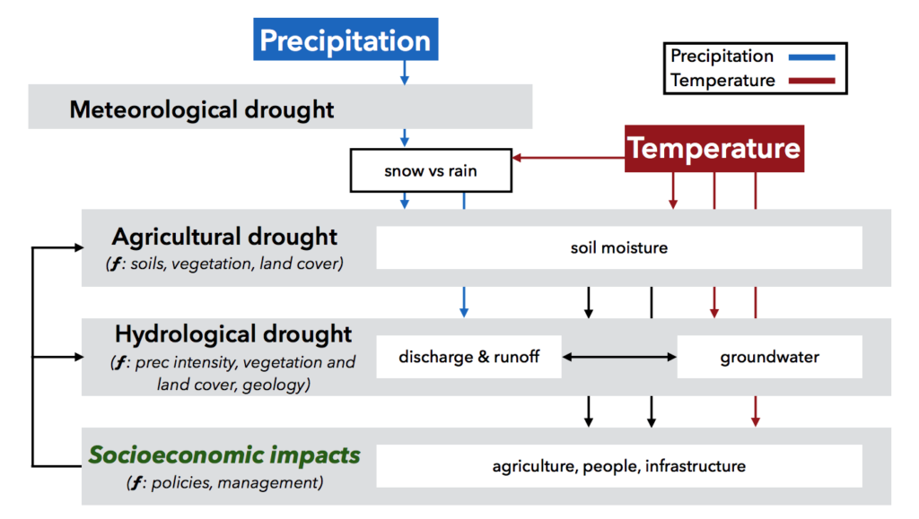
Schematic illustrating the classical definitions of drought and the associated processes. Precipitation deficits are the ultimate driver of most drought events, with these deficits propagating over time through the hydrological cycle. Other climate variables, particularly temperature, can also affect both agricultural and hydrological drought. Credit: Cook et al. (2018)
The above definitions show that drought is rarely about precipitation – rain, hail, sleet and/or snow – alone. Warmer temperatures, for example, can increase evaporation of moisture from the surface, increase the fraction of precipitation falling as rain rather than snow, and advance the timing of the snow melt season in spring. Vegetation, soil type and topography can all affect droughts through the way they intercept and hold (or do not hold) rainwater.
Humans also play a key role through how we use water (irrigating farmland and withdrawing water from long-held groundwater sources, for example) and change the land surface through deforestation, expanding croplands and urban development.
Because there are many ways to define a drought, there are also numerous ways to quantify one. These “indices” take into account different variables that can be measured directly or indirectly, such as precipitation, temperature, evaporation, soil moisture, river flows and reservoir levels.
One of the most common, for example, is the Palmer Drought Severity Index (PDSI). This uses monthly estimates of evapotranspiration (calculated largely as a function of temperature) and rainfall data, as well as information on the water-holding capacity of the soil.
It is also possible to use more than one drought indicator. For example, the US Drought Monitor classifies drought severity according to a combination of five different indices (including PDSI), along with drought impacts and local reports from expert observers. As the map below shows, this gives a score of drought intensity and impacts from “D0 – Abnormally dry” (yellow shading) up to “D4 – Exceptional Drought” (maroon).
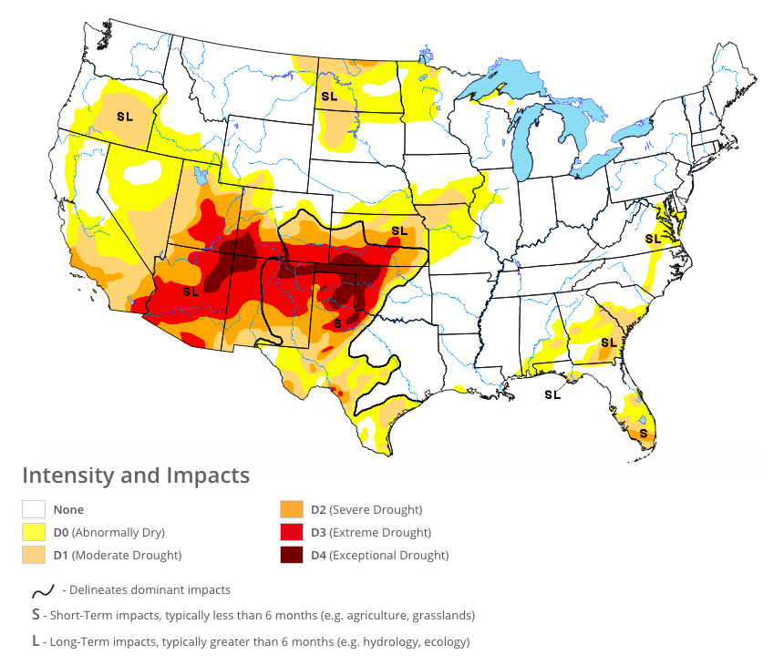
Drought severity across the US as of 10 May. Intensity of drought indicated by colour of shading, from none (white) through to exceptional drought (maroon). Credit: US Drought Monitor
Detection and attribution
The multitude of contributing factors to a drought means that identifying the sometimes-subtle signal of climate change is tricky.
In part because of this, the fifth assessment report of the Intergovernmental Panel on Climate Change (IPCC) in 2013 concluded that there was low confidence (pdf) that any significant trends in drought could be detected or attributed to climate change.
Since then, however, the science of detection and attribution – concerned with identifying changes in the climate system and their causes – has advanced considerably.
Findings from more recent studies using state-of-the-art models and techniques have significantly advanced our understanding of drought and climate change. These studies, using climate models, the observational record and palaeoclimate information, have clearly demonstrated that climate change has played a role in recent droughts.
In the Mediterranean, for example, declines in rainfall driven by climate change have increased drought risk across the region, amplifying recent events including the drought that preceded the Syrian civil war.
Along the Pacific coast of the US, warmer temperatures from climate change have pushed snow and soil moisture to record breaking deficits in California and the Pacific Northwest. In the Upper Colorado river basin, warmer temperatures have even caused significant river flow deficits, despite near normal levels of precipitation.
A climate change signal has not been detected with confidence for every drought, especially in regions where natural climate variability is more complex or less well understood – in Australia and East Africa, for example. But for many places, the fingerprints of climate change are undeniably clear.
Projecting precipitation
With climate change already having an impact on droughts, we can reasonably expect this impact to increase as the climate warms further. And model projections bear this out.
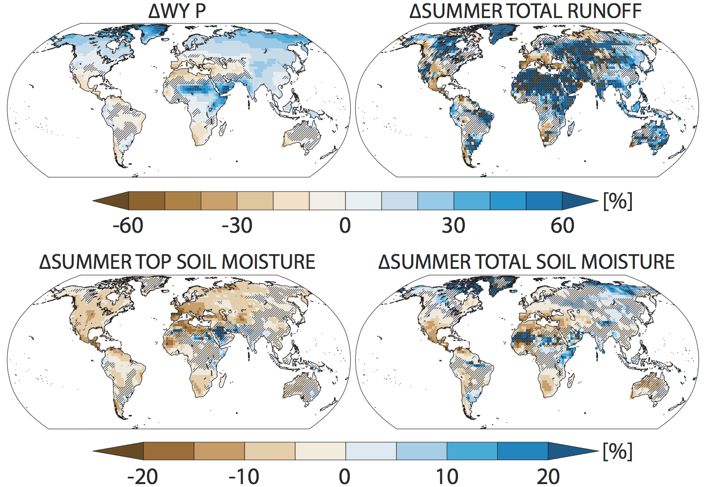
The maps below give some examples according to simulations under a high warming scenario (“RCP8.5”) using 17 climate models. They show the projected percentage change in annual rainfall (top left), summer rainfall runoff (top right), summer soil moisture in the top 10cm (bottom left) and summer total column soil moisture (various depths for different models; bottom right) between 1976-2005 and 2070-99. “Runoff” is the amount of rainfall that flows over land into streams and rivers rather than soaking into the ground.
The colour of the shading indicates whether an area is likely to get wetter (blue) or drier (brown).

End-of-century percentage changes in hydroclimate variables from 17 models in the CMIP5 archive (2070-2099 minus 1976-2005) under RCP8.5. Moving clockwise from the upper left: water-year (WY; October–September in the northern hemisphere and July–June in the Southern Hemisphere) precipitation (P), summer (June-July-August in the northern hemisphere; December-January-February in the southern hemisphere) total runoff, summer near surface soil moisture (0.1m), and summer full-column soil moisture. In all panels, drying tendencies are indicated in brown, wetting tendencies in blue. Hatching shows areas will little agreement between model results. Amended from Cook et al. (2018)
Although projections generally agree a little less across models for rainfall changesthan for temperature, they do show – unequivocally – an increased drying and drought risk for many regions of the world.
Most likely to be adversely affected are Mediterranean regions of Europe and Africa, Central America, southwest US and the subtropics of the southern hemisphere.
This drying occurs because of climate change-forced regional declines in rainfall, but also from the direct effect of warmer temperatures, which increases evaporative losses from the surface, causes earlier snowmelt and shifts precipitation from snow to rain.
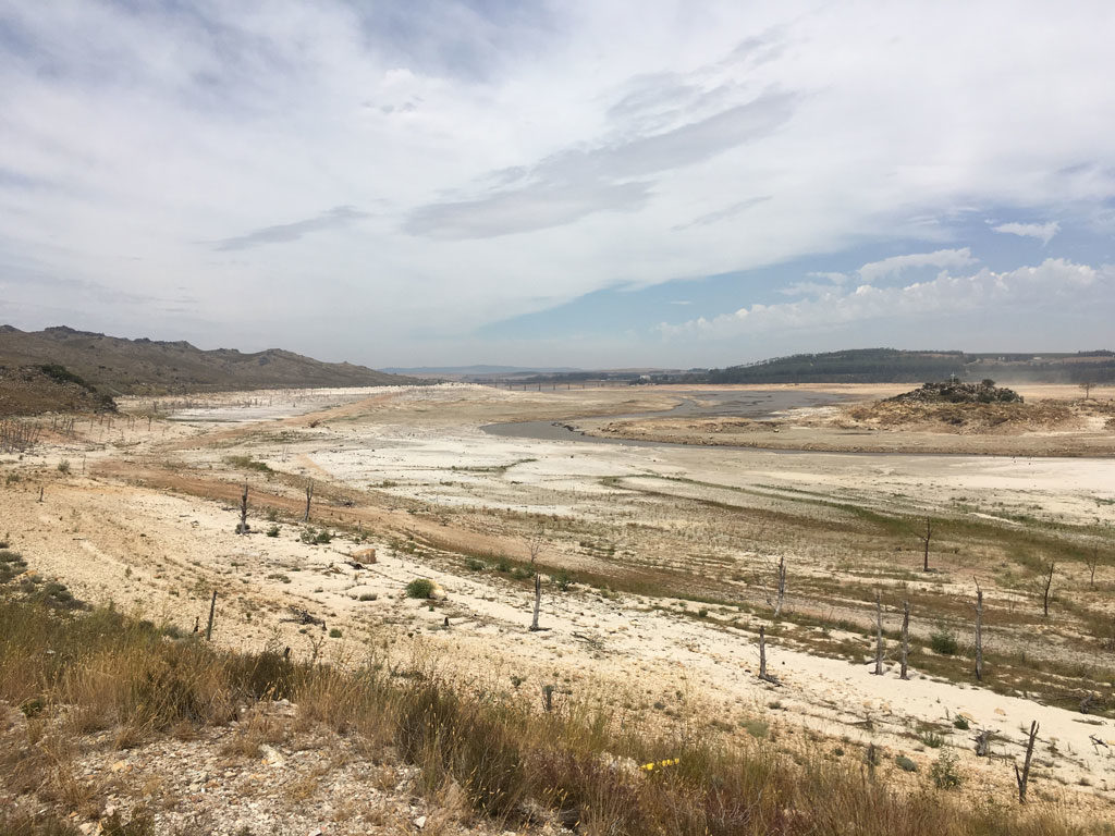
Theewaterskloof Dam, the biggest reservoir for Cape Town, in February 2018. Credit: Robert McSweeney
Consequently, significant drying in the future is expected to affect large regions in the subtropics and mid-latitudes, even in areas where rainfall changes are negligible.
When rainfall does occur, it is more likely to be in shorter, more intense bursts. This might mean summers are increasingly likely to see periods of dry weather punctuated with heavy storms. As a result, summer runoff may actually increase for many areas because of more intense rains. While this might be beneficial for topping up rivers, lakes and reservoirs, it does not necessarily help relieve soil moisture deficits and groundwater shortages.
Challenges and opportunities
While a drier future – and, in some cases, present – poses significant challenges for the management of water resources, there are also substantial opportunities to alleviate the worst impacts.
These include policies for improving water conservation and stakeholder cooperation, exploiting surpluses during wet years (which still occur, even in the driest projections), and the clear benefits of cutting greenhouse gases for limiting the extent of climate change and reducing drought risk in many regions.
While studies of the physical climate system cannot provide recommendations for one path or the other, they do highlight the challenges that will be necessary to address in a world that will be warmer – and, in many places, drier – than anything humanity has experienced in the last 200 years.
Cook, B. I., et al. (2018) Climate Change and Drought: From Past to Future, Current Climate Change Reports, doi:10.1007/s40641-018-0093-2
from Skeptical Science https://ift.tt/2GI7Zei
This is a re-post from Carbon Brief by Benjamin Cook
Dr Benjamin Cook is a climate scientist at the NASA Goddard Institute for Space Studies and the Lamont-Doherty Earth Observatory.
Few areas of the world are completely immune to droughts and their often-devastating impacts on water resources, ecosystems and people.
Regions as diverse as California, the Eastern Mediterranean, East Africa, South Africa and Australia have all experienced severe – and, in some cases, unprecedented – droughts in recent years.
As with other climate and weather extremes, such as storms and floods, these events have spurred strong interest in questions surrounding the impact of climate change. For example, is climate change making droughts more frequent or severe? And can we expect climate change to contribute to increased drought risk and severity in the future?
The most recent research shows climate change is already making many parts of the world drier and droughts are likely to pack more punch as the climate warms further.
Defining drought
Droughts are among the most expensive weather-related disasters in the world (pdf), affecting ecosystems, agriculture and human society.
The scale of the impacts underlines how important it is to understand droughts and how their likelihood and severity can be made worse by climate change.
But this is easier said than done. For a start, drought is fundamentally a cross-disciplinary phenomenon – it extends across the fields of meteorology, climatology, hydrology, ecology, agronomy, and even sociology, economics, and anthropology.
This means how you define a drought may depend on your field of interest.
A meteorologist might characterise a drought as a straightforward lack of rainfall (known as “meteorological drought”). A farmer, however, would be most concerned when the lack of rain affects soil moisture and crop growth (“agricultural drought”). While a hydrologist would be most interested in when this has a noticeable impact on river flows, aquifers and surface reservoirs (“hydrological drought”).
Schematic illustrating the classical definitions of drought and the associated processes. Precipitation deficits are the ultimate driver of most drought events, with these deficits propagating over time through the hydrological cycle. Other climate variables, particularly temperature, can also affect both agricultural and hydrological drought. Credit: Cook et al. (2018)
The above definitions show that drought is rarely about precipitation – rain, hail, sleet and/or snow – alone. Warmer temperatures, for example, can increase evaporation of moisture from the surface, increase the fraction of precipitation falling as rain rather than snow, and advance the timing of the snow melt season in spring. Vegetation, soil type and topography can all affect droughts through the way they intercept and hold (or do not hold) rainwater.
Humans also play a key role through how we use water (irrigating farmland and withdrawing water from long-held groundwater sources, for example) and change the land surface through deforestation, expanding croplands and urban development.
Because there are many ways to define a drought, there are also numerous ways to quantify one. These “indices” take into account different variables that can be measured directly or indirectly, such as precipitation, temperature, evaporation, soil moisture, river flows and reservoir levels.
One of the most common, for example, is the Palmer Drought Severity Index (PDSI). This uses monthly estimates of evapotranspiration (calculated largely as a function of temperature) and rainfall data, as well as information on the water-holding capacity of the soil.
It is also possible to use more than one drought indicator. For example, the US Drought Monitor classifies drought severity according to a combination of five different indices (including PDSI), along with drought impacts and local reports from expert observers. As the map below shows, this gives a score of drought intensity and impacts from “D0 – Abnormally dry” (yellow shading) up to “D4 – Exceptional Drought” (maroon).
Drought severity across the US as of 10 May. Intensity of drought indicated by colour of shading, from none (white) through to exceptional drought (maroon). Credit: US Drought Monitor
Detection and attribution
The multitude of contributing factors to a drought means that identifying the sometimes-subtle signal of climate change is tricky.
In part because of this, the fifth assessment report of the Intergovernmental Panel on Climate Change (IPCC) in 2013 concluded that there was low confidence (pdf) that any significant trends in drought could be detected or attributed to climate change.
Since then, however, the science of detection and attribution – concerned with identifying changes in the climate system and their causes – has advanced considerably.
Findings from more recent studies using state-of-the-art models and techniques have significantly advanced our understanding of drought and climate change. These studies, using climate models, the observational record and palaeoclimate information, have clearly demonstrated that climate change has played a role in recent droughts.
In the Mediterranean, for example, declines in rainfall driven by climate change have increased drought risk across the region, amplifying recent events including the drought that preceded the Syrian civil war.
Along the Pacific coast of the US, warmer temperatures from climate change have pushed snow and soil moisture to record breaking deficits in California and the Pacific Northwest. In the Upper Colorado river basin, warmer temperatures have even caused significant river flow deficits, despite near normal levels of precipitation.
A climate change signal has not been detected with confidence for every drought, especially in regions where natural climate variability is more complex or less well understood – in Australia and East Africa, for example. But for many places, the fingerprints of climate change are undeniably clear.
Projecting precipitation
With climate change already having an impact on droughts, we can reasonably expect this impact to increase as the climate warms further. And model projections bear this out.
The maps below give some examples according to simulations under a high warming scenario (“RCP8.5”) using 17 climate models. They show the projected percentage change in annual rainfall (top left), summer rainfall runoff (top right), summer soil moisture in the top 10cm (bottom left) and summer total column soil moisture (various depths for different models; bottom right) between 1976-2005 and 2070-99. “Runoff” is the amount of rainfall that flows over land into streams and rivers rather than soaking into the ground.
The colour of the shading indicates whether an area is likely to get wetter (blue) or drier (brown).
End-of-century percentage changes in hydroclimate variables from 17 models in the CMIP5 archive (2070-2099 minus 1976-2005) under RCP8.5. Moving clockwise from the upper left: water-year (WY; October–September in the northern hemisphere and July–June in the Southern Hemisphere) precipitation (P), summer (June-July-August in the northern hemisphere; December-January-February in the southern hemisphere) total runoff, summer near surface soil moisture (0.1m), and summer full-column soil moisture. In all panels, drying tendencies are indicated in brown, wetting tendencies in blue. Hatching shows areas will little agreement between model results. Amended from Cook et al. (2018)
Although projections generally agree a little less across models for rainfall changesthan for temperature, they do show – unequivocally – an increased drying and drought risk for many regions of the world.
Most likely to be adversely affected are Mediterranean regions of Europe and Africa, Central America, southwest US and the subtropics of the southern hemisphere.
This drying occurs because of climate change-forced regional declines in rainfall, but also from the direct effect of warmer temperatures, which increases evaporative losses from the surface, causes earlier snowmelt and shifts precipitation from snow to rain.
Theewaterskloof Dam, the biggest reservoir for Cape Town, in February 2018. Credit: Robert McSweeney
Consequently, significant drying in the future is expected to affect large regions in the subtropics and mid-latitudes, even in areas where rainfall changes are negligible.
When rainfall does occur, it is more likely to be in shorter, more intense bursts. This might mean summers are increasingly likely to see periods of dry weather punctuated with heavy storms. As a result, summer runoff may actually increase for many areas because of more intense rains. While this might be beneficial for topping up rivers, lakes and reservoirs, it does not necessarily help relieve soil moisture deficits and groundwater shortages.
Challenges and opportunities
While a drier future – and, in some cases, present – poses significant challenges for the management of water resources, there are also substantial opportunities to alleviate the worst impacts.
These include policies for improving water conservation and stakeholder cooperation, exploiting surpluses during wet years (which still occur, even in the driest projections), and the clear benefits of cutting greenhouse gases for limiting the extent of climate change and reducing drought risk in many regions.
While studies of the physical climate system cannot provide recommendations for one path or the other, they do highlight the challenges that will be necessary to address in a world that will be warmer – and, in many places, drier – than anything humanity has experienced in the last 200 years.
Cook, B. I., et al. (2018) Climate Change and Drought: From Past to Future, Current Climate Change Reports, doi:10.1007/s40641-018-0093-2
from Skeptical Science https://ift.tt/2GI7Zei