In Part I of this look back at 1970s climate science I reviewed the findings of Peterson, Connolley, and Fleck's seminal 2008 survey of 1970s peer-reviewed literature (hereafter referred to as PCF08) which found no 1970s "consensus" about a future global cooling/ice age. I also looked at a "skeptic" critique of this paper from the blogsite No Tricks Zone, penned by Kenneth Richard (hereafter referred to as NTZ), and showed some of the errors and fallacies he used to distort 1970s science. In this post I'll take a closer look at some of the papers used by NTZ to claim that there was a global cooling "consensus" in the 1970s.
The primary critique by NTZ is given in a blog post which highlights 35 "sample global cooling/low CO2 climate influence papers" from his full list of 285 papers. Like the full list of 285 papers, these samples are not given in any apparent order, not by date or by author. I rearranged these by date of publication in order to see the progression of the science as the various threads of climate research (see Part I) developed throughout the period. Below is a screenshot of the first page of a spreadsheet (click on image for pdf) of the 35 sample papers.
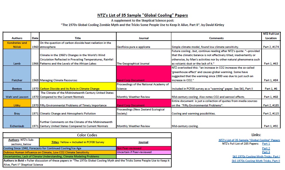
The first thing to notice is that not all of these samples are peer-reviewed scientific papers. Two of these are RAND Corporation documents (Fletcher, 1969 and Libby, 1970), one is a book review (Post, 1979), and one is from a popular science magazine (Douglas, 1975). This article was mentioned in PCF08 in their "Popular Literature of the Era" sidebar but not included in their survey. Two other sample papers are perhaps "borderline" between grey and peer-reviewed literature: two Master's thesis papers (Cimorelli & House, 1974 and Magill, 1980). And there are a few others I'm not sure about.
Contrast this with PCF08's survey which excluded anything from the "grey literature" and focused exclusively on the peer-reviewed literature.1 The best place to find out what the scientists of the time were saying about the future climate trajectory is in the peer-reviewed literature. Things can get muddy once you include documents from the popular press. Yes, these other sources may offer insight into what the "sense of the times" were, but they can also misrepresent or distort what scientists thought at the time. NTZ expands the goal posts to include some of this grey literature and thus gathers more "papers" for his "global cooling consensus".
A detailed examination of NTZ's sample list of 35 papers is beyond the scope of this blog post (see pdf of spreadsheet above for further details on papers not discussed in this post). Instead, I will focus on some examples to illustrate the ways NTZ misrepresents 1970s climate science.
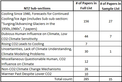
The table above shows the sub-sections which NTZ used to organize his pile of papers. In the sample list, the papers are in the two most-numerous categories: "Cooling Since 1940..." and "Dubious Human Influence...", and there is one paper from the sub-section, "Uncertainties...". By far, most papers in the full NTZ list (as well as the sample list) are found in the sub-section: "Cooling Since 1940, Forecasts for Continued Cooling/Ice Age". As pointed out in Part I, NTZ shifts the focus from PCF08's look to future climate projections to a view of what scientists were saying about the recent mid-century cooling trend.
NTZ's Cooling Category
Benton 1970, a short two-page paper, succinctly lays out some of the main threads of 1970s climate science. Benton notes the rise of global temperatures at the beginning of the 20th century, followed by the mid-century cooling trend. He discusses CO2's impact on climate and then aerosol's (both volcanic and human) possible cooling and/or warming impacts. PCF08 included this paper in their survey in their "warming" category, perhaps because of this quote:
Recent numerical studies have indicated that a 10% increase in carbon dioxide should result, on average, in a temperature increase of about 0.3°C at the earth's surface. The present rate of increase of 0.7 ppm per year would therefore (if extrapolated to 2000 A.D.) result in a warming of about 0.6°C—a very substantial change.
NTZ ignores this clear prediction and only zeros in on what the paper says about mid-century cooling. This cherry picking, or selective quoting, is by far NTZ's most used technique.
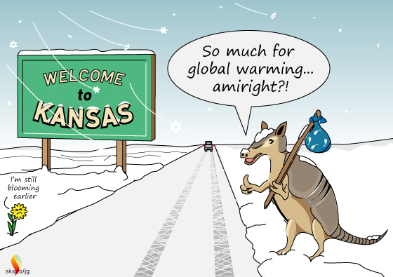
Almost any paper which mentions the mid-century cooling, no matter how tangentially, is added to NTZ's pile of papers. Schultz 1972 is about climatic impacts on Holocene mammal migrations. He discusses how armadillos expanded their North American range northwards during the first half of the 20th century, but are now, in 1972, headed back south:
The armadillos, however, appear to have disappeared from their lately acquired northern range, and now seem to be found chiefly south of the central part of Kansas. This change in distribution has taken place during the past 10 yr, when the winters have been longer and colder.
That's it. The main focus of the paper is on trying to see if changes in the ranges of other late Pleistocene and Holocene mammals might also be due to climate changes. It looks at the present armadillo migrations as a possible analog of the past, and says nothing about future climate trajectory.
One of the few papers that actually forecast a future ice age is Kukla 1972, as quoted by NTZ: "A new glacial insolation regime, expected to last 8000 years, began just recently. Mean global temperatures may eventually drop about 1°C in the next hundred years." This paper may be the only example of a "cooling" paper missed by the PCF08 survey and found by NTZ.
Kukla 1972 is also one of the few papers that deals with that other thread of 1970s climate science: Milankovitch cycles. Kukla showed how past changes in orbital cycles very slightly altered the amount of solar energy hitting the Earth, leading to past glacial and interglacial periods. Kukla rightly noted that the "change in the heat income due to Milankovitch mechanism is so minute that it cannot lead directly to glaciation or deglaciation...Only when multiplied by some efficient feedback mechanism can the insolation trigger climatic change". One of the main feedbacks is from changes in the Earth's albedo. At the start of a glacial period, as more and more ice accumulates in the polar regions, more and more incoming solar radiation is reflected from the growing ice fields, which leads to further cooling.
Besides looking back to past ice ages, Kukla also extrapolated the orbital cycles into the future to forecast continued cooling and a descent into another ice age. But Kukla stressed that his extrapolation was "still today [a] somewhat speculative" estimate.
This paper is from a symposium held in 1974 on atmospheric pollution, and so it may not technically be "peer-reviewed". The NTZ quote from this paper mentions that there had been "a flood of papers" dealing with the "exponentially increasing pollution". Ellsaesser notes that "the particulate increases were usually cited as at least contributing to the post 1940 cooling and possibly capable of bringing on another ice age". But a full reading of the paper shows that the entire point of Ellsaesser's paper is to counter that argument. He complains about the environmental alarmism of the day concerning pollution and cooling. And, ironically, he complains that not enough emphasis is given to CO2:
Of the climatic problems raised, the CO2 one is best understood. There is essentially universal agreement that atmospheric CO2 is increasing as a result of the consumption of fossil fuels and that this should enhance the 'greenhouse' effect leading to a warming of the planetary surface. The strongest support for the upward trend in air-borne particulates derives from the failure of observational data to support our understanding of the CO2 effect. Yet no one ever hears the argument that man might consider a deliberate increase in particulates to counter the CO2 effect or alternatively that the CO2 effect is just what is needed to prevent or delay the onset of the next glacial advance which is now imminent according to students of this problem.
NTZ put this paper in his "cooling" sub-section, but a better fit would probably be in his "dubious human influence..." sub-section. Robock used a simple energy balance model to investigate how various forcings, both natural and anthropogenic, may have influenced global temperatures from about the 1880s to the 1960s. For the natural forcings Robock made various runs using different solar forcings and two runs using different volcanic aerosol numbers. For the anthropogenic forcings he used one run each for CO2, aerosols, and "heat". Robock found that the forcing which most closely mirrored the actual temperature observations was volcanic aerosols: "volcanic dust is the only external forcing that produces a model response significantly like the observations".
Robock only modelled each forcing separately, not in combination. But he did note that some of these forcings, working in tandem in the real world, could possibly explain the observed temperature record of the past ~100 years.
What about CO2 and anthro-aerosols? His model showed a slight warming from CO2 and a slight cooling from human pollution, not enough to really matter, and when combined they essentially cancelled each other out. NTZ's quote from the paper highlights this fact: "One could sum the anthropogenic effects for each region, which would show almost no effect in the NH [Northern Hemisphere] and warming in the SH [Southern Hemisphere]." But he ignores the following sentence: "Drawing conclusions from this exercise would not be meaningful, however, due to our lack of understanding of the aerosol effect." Robock also pointed out:
All the effects [of human forcings] almost double every 20 years. They are not of sufficient magnitude to have much effect on the observational records, which end about 1960, but may have a measurable effect in the near future.
The relative magnitudes of the effects may change in the future due to changing human pollution policies. Restrictions on particulate pollution and anticipated measures against sulfate aerosols will lessen the effects of industrial aerosols.
Indeed, this is what actually happened. Clean Air rules lessened particulate/aerosol pollution but did nothing to limit CO2 emissions. The cooling effect of aerosols never materialized but the warming effect of CO2 has steadily risen since Robock's simple model runs.
This paper is a "case study" which looked at the mid-century cooling in Indiana, specifically in the summer months (June, July, and August) since the authors were also interested in any change in climate during the growing season. When scientists in the 1960s-70s compiled data to build their global average temperature series they used state averages of monthly mean temperatures from weather stations around the world. Nelson et al. noted that:
any changes in location of stations and time of observation were tacitly assumed to be random and to have little effect on divisional and state mean temperature records. Schaal and Dale (1977), however, showed that in Indiana a systemic change in the time that observations were taken at cooperative climatological stations--from evening to morning--contributed to the downward trend observed in divisional and state mean temperatures since 1970. [Italics in original.]
Was the mid-century cooling really just an artifact of changes in temperature recording methods which made it seem like the globe was cooling? Nelson et al took a closer look at the Indiana data and made adjustments to correct for any biases. Their corrections got rid of some of the mid-century cooling, but not all of it.
Of course, this is just summer months in Indiana, not a global view of temperature changes. But it shows the care and precision used by scientists who did the early work of building an accurate record of global temperatures. I'm surprised that NTZ included this paper in his collection because usually "skeptics" tend to dislike "temperature adjustments" (see here and here). I guess it is okay as long as those adjustments still show cooling.
The last paper I'll look at from this sub-category is about a changing "diurnal temperature range" or DTR. Here is NTZ's quote:
An appreciable number of nonurban stations in the United States and Canada have been identified with statistically significant (at the 90% level) decreasing trends in the monthly mean diurnal temperature range between 1941-80.
I think NTZ likes this paper because it mentions "decreasing trends" and "temperature" in the first sentence of the paper's abstract. But, I don't think he understands what "decreasing trends in monthly mean diurnal temperature range" means. The DTR is merely the "difference between the maximum and minimum temperature during a 24-hour period" (IPCC). The "decreasing trend" discussed in this paper refers to a decrease in the range between the maximum and minimum daily temperatures.
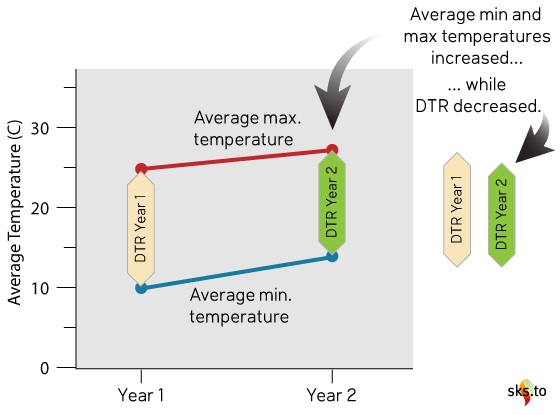
For example (see figure above), let's say the average monthly max. temp. at some location was 25°C and the min. temp. was 10°C, the range would be 15°C. Now, at some later time, if the max. temp. is 27°C and the min. temp. is 14°C, then the DTR would be 13°C. Hence, the DTR has decreased from 15 to 13°C. Notice in this example the average temperatures went up but the DTR went down. Also notice the min. temps increased slightly more than the max. temps.
Why would scientists study DTR? In the abstract, Karl et al say:
The physical mechanism responsible for the observed decrease in the diurnal range is not known. Possible explanations include greenhouse effects such as changes in cloudiness, aerosol loading, atmospheric water vapor content, or carbon dioxide.
They also pointed out that the specific nature of the decreasing DTR they found also points to an enhanced greenhouse effect:
An increased greenhouse effect due to humidity, CO2, aerosols or clouds is expected to produce a relative increase of the minima with respect to the maxima and a decrease of the diurnal range. The reported observations are consistent with the hypothesized changes.
Even today, the jury is still not settled on weather a decreasing DTR is a solid "fingerprint" of an enhanced CO2-greenhouse warming. But Karl et al was one of the papers from the 1970s (actually 1980s!) which offered support for this idea, and had nothing to do with cooling (mid-century or in a future ice age).
NTZ's Dubious Human Influence Category
This is another rare paper in NTZ's collection which actually had a prediction about an "imminent"3 ice age. It is also one of the many PCF08 papers which NTZ repurposed: PCF08 had categorized it as "neutral". But NTZ's selected quote4 ignored any mention of a future ice age and zeroed in on Willett's dismissal of CO2's influence on recent climate:
[T]he author is convinced that recent increases of atmospheric carbon dioxide have contributed much less than 5% of the recent changes of atmospheric temperature, and will contribute no more than that in the foreseeable future.
Willett also didn't think that particulate/aerosol/dust pollution would have much effect. He preferred a solar influence hypothesis and concluded that there was no "imminent" ice age coming:
There is no other reason to anticipate an Ice Age in the near future. It is the author's contention that. 1. The pollution hypotheses [CO2 or dust/aerosols] cannot properly be made to account for recent climatic fluctuations. 2. The solar hypothesis appears to fit the observed pattern of climatic fluctuation in much greater detail, and does not call for an imminent Ice Age.
And to drive home the point, Willett said it was his "final conclusion that man will pollute himself off the face of the earth long before he can pollute himself into an Ice Age".
Well, actually, here is his final conclusion, just in case the reader wasn't paying attention:
The author's reasoned answer, then, to the question, 'Do Recent Climatic Fluctuations Portend an Imminent Ice Age?' is an emphatic NO...the next Ice Age is unlikely for at least 10,000 years, more likely for more than 30,000 years, unless the sun takes off on a new tangent. [Emphasis in the original]
NTZ ignored all of these clear predictions about a future ice age and instead he focused on Willett's views, since shown to be wrong, about CO2's "dubious influence" on climate.
Here is NTZ's selected quote from this paper:
The measured increase in carbon dioxide in the atmosphere, according to the most recent computations, would not be enough to have any measurable climatic effect.
The very next part of this quote is:
Rasool and Schneider (1971) conclude that an increase in the carbon dioxide content of eight times the present level would produce an increase in surface temperature of less than 2°C, and that if the concentration were to increase from the present level of 320 parts per million to about 400 by the year 2000, the predicted increase in surface global temperature would be about 0.1°C
Rasool and Schneider (1971) (hereafter: R&S71) is one of the seminal climate papers from the 1970s, and PCF08 categorized it as one of their seven "cooling" papers. PCF08 stated that this paper "may be the most misinterpreted and misused paper in the story of global cooling". R&S71 was one of the first studies using modeling, and their results found minimal warming effects from CO2 and large cooling effects from aerosols. But other scientists, and even Rasool and Schneider, quickly noticed flaws in R&S71 (Charlson et al 1972 and Rasool and Schneider 1972). Further improvements in 1975 (this time by Schneider and Mass) showed that R&S71 "had overestimated cooling [from aerosols] while underestimating the greenhouse warming contributed by carbon dioxide" (PCF08).
Dunbar's paper was published one year after Schneider and Mass's corrections to R&S71, but no corrections to R&S71 are noted in Dunbar's paper, he still used the incorrect results. Perhaps Dunbar can be excused for this oversight since the corrections were still very new. But, when we look back at these papers we should be mindful of the larger context of the science of the time, and recognize when a "money quote" may require further research.
A few years after Dunbar, Barrett 1978 also used R&S71 without noting the corrections, but he also referenced enough of the other relevant literature to arrive at a more accurate estimate of CO2's effect. The result is a good overview of the state of the science in the 1970s.
Still, NTZ was able to find a quote which seemed to downplay man's influence on climate:
In particular, detection of an anthropogenic influence through statistical analysis alone requires a long run of data of good quality and careful attention to measures of significance. It is most important to avoid the post hoc ergo propter hoc fallacy that a trend of a few years’ duration or less, following some change in human activities, can be attributed to that change even when no sound physical causal relationship is evident. [Emphasis in the original.]
Conveniently, NTZ avoided the rest of the paper which went on to describe the "sound physical causal relationship[s]" between CO2, aerosols, and climate. In the concluding remarks of the paper, Barrett predicted that atmospheric CO2 would rise to "between 350 and 415 ppmv by the end of the [20th] century". The actual value in 2000 was about 368 ppm, well within the predicted range.
Barrett also predicted that this increase in CO2 "should increase the temperature by 0.3°C; this trend might be detectable by careful analysis unless it is offset by other effects, such as those of aerosols". Careful analysis by NASA-GISS, NOAA, HadCRU, and JMA (as well as others) have shown that this prediction was also remarkably accurate, if not a bit low (see figure below).
 Global surface temperature anomalies from NASA-GISS, HadCRU, NOAA, and JMA. I've circled in red the 1970s, which are centered on the zero baseline. The vertical red line indicates the year 2000, and the two horizontal lines demarcate the temp. anomaly range from 0.3 to 0.5°C. (Source: NASA-GISS.)
By the year 2000, global average temperatures had risen about 0.3 to 0.5°C since the 1970s. And they haven't stopped there. There's no global cooling in sight.
The Rich Tapestry of Climate Science
Science is a process of making observations of the natural world, gathering data, asking questions, and performing experiments—all to get a clear picture of how the world works. This picture—or description, or model—can only be clear if it includes as much information as possible about the real world. If information is left out, our model of how the world works will be incomplete. Some incompleteness is inevitable because we can never have all of the relevant information, and the information we do have will never be "perfect".
NTZ's description of 1970s climate science focused heavily on the mid-century cooling trend in global average temperatures, and on studies which downplayed CO2's role in the greenhouse effect. This is hardly a complete picture of 1970s science, nor does it give us a very good model of the climate system (as understood by 1970s scientists). NTZ arrived at his "cooling consensus" by often just selecting quotes which supported his view. But, a thorough reading of these papers reveals the full breadth of 1970s science.
In some papers, researchers might look at the mid-century cooling trend and hypothesize that aerosols may have caused it, and then they may look at what possible effects aerosols might have on future climate. The very same paper may also make note of CO2's warming influence, and on possible outcomes if atmospheric CO2 continues to increase in the future. Benton 1970 and Barrett 1978 both fit this description. But if you just read NTZ's quotes from these papers you would know nothing about forecasts of future warming.
NTZ's goal-post shifting, straw-man arguments, and quote mining/cherry picking result in a lopsided description of 1970s climate science. It is possible to get a more accurate description of what scientists knew (and didn't know) about climate in the 1970s from NTZ's pile of papers. But to do so you have to read beyond the selected "money quotes" and look at all of the data. When you do so, you won't find a majority of 1970s scientists forecasting "global cooling". Instead you will find what PCF08 found in their literature review:
[P]erhaps more important than demonstrating that the global cooling myth is wrong, this review shows the remarkable way in which the individual threads of climate science of the time—each group of researchers pursuing their own set of questions—was quickly woven into the integrated tapestry that created the basis for climate science as we know it today.
Thanks to jg for the illustrations, and to BaerbelW for help with the spreadsheet.
Footnotes
1. PCF08 did make a few exceptions for "prestigious reports": "The gray literature of conference proceedings were not authoritative enough to be included in the literature search. However, a few prestigious reports that may not have been peer reviewed have been included in this literature survey because they clearly represent the science of their day."
2. NTZ has incorrect date of 1975 for this paper.
3. Willett is very specific about the term "imminent": it refers "to one or at most two centuries in the future".
4. It is worth looking at the longer quote from Willett in NTZ's full list to see another example of NTZ's confused counting, as described in Part I. Willett is listed as #158 in the Part 2 list. A screenshot of this is shown below.
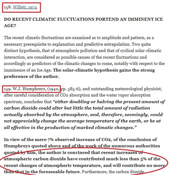
NTZ gives the title of Willett's paper and then a single paragraph. Then there is the next listing: #159 - Humphreys (1940). But the paragraph from Willett here doesn't contain the shorter quote given in NTZ's list of 35 papers. The actual shorter quote from the "35" list is circled in the screenshot (starting with "the author is convinced...". But isn't that from Humphreys? No, all three of these paragraphs are from Willett: the first is from the abstract and the other two are from the paper (p. 273). NTZ has simply added a new listing number (#159) to the quoted material from Humphreys (1940) used by Willett! Now the expanded time span for NTZ's "1970s" climate science extends back to 1940!
from Skeptical Science https://ift.tt/2FXlTsC
In Part I of this look back at 1970s climate science I reviewed the findings of Peterson, Connolley, and Fleck's seminal 2008 survey of 1970s peer-reviewed literature (hereafter referred to as PCF08) which found no 1970s "consensus" about a future global cooling/ice age. I also looked at a "skeptic" critique of this paper from the blogsite No Tricks Zone, penned by Kenneth Richard (hereafter referred to as NTZ), and showed some of the errors and fallacies he used to distort 1970s science. In this post I'll take a closer look at some of the papers used by NTZ to claim that there was a global cooling "consensus" in the 1970s.
The primary critique by NTZ is given in a blog post which highlights 35 "sample global cooling/low CO2 climate influence papers" from his full list of 285 papers. Like the full list of 285 papers, these samples are not given in any apparent order, not by date or by author. I rearranged these by date of publication in order to see the progression of the science as the various threads of climate research (see Part I) developed throughout the period. Below is a screenshot of the first page of a spreadsheet (click on image for pdf) of the 35 sample papers.
The first thing to notice is that not all of these samples are peer-reviewed scientific papers. Two of these are RAND Corporation documents (Fletcher, 1969 and Libby, 1970), one is a book review (Post, 1979), and one is from a popular science magazine (Douglas, 1975). This article was mentioned in PCF08 in their "Popular Literature of the Era" sidebar but not included in their survey. Two other sample papers are perhaps "borderline" between grey and peer-reviewed literature: two Master's thesis papers (Cimorelli & House, 1974 and Magill, 1980). And there are a few others I'm not sure about.
Contrast this with PCF08's survey which excluded anything from the "grey literature" and focused exclusively on the peer-reviewed literature.1 The best place to find out what the scientists of the time were saying about the future climate trajectory is in the peer-reviewed literature. Things can get muddy once you include documents from the popular press. Yes, these other sources may offer insight into what the "sense of the times" were, but they can also misrepresent or distort what scientists thought at the time. NTZ expands the goal posts to include some of this grey literature and thus gathers more "papers" for his "global cooling consensus".
A detailed examination of NTZ's sample list of 35 papers is beyond the scope of this blog post (see pdf of spreadsheet above for further details on papers not discussed in this post). Instead, I will focus on some examples to illustrate the ways NTZ misrepresents 1970s climate science.
The table above shows the sub-sections which NTZ used to organize his pile of papers. In the sample list, the papers are in the two most-numerous categories: "Cooling Since 1940..." and "Dubious Human Influence...", and there is one paper from the sub-section, "Uncertainties...". By far, most papers in the full NTZ list (as well as the sample list) are found in the sub-section: "Cooling Since 1940, Forecasts for Continued Cooling/Ice Age". As pointed out in Part I, NTZ shifts the focus from PCF08's look to future climate projections to a view of what scientists were saying about the recent mid-century cooling trend.
NTZ's Cooling Category
Benton 1970, a short two-page paper, succinctly lays out some of the main threads of 1970s climate science. Benton notes the rise of global temperatures at the beginning of the 20th century, followed by the mid-century cooling trend. He discusses CO2's impact on climate and then aerosol's (both volcanic and human) possible cooling and/or warming impacts. PCF08 included this paper in their survey in their "warming" category, perhaps because of this quote:
Recent numerical studies have indicated that a 10% increase in carbon dioxide should result, on average, in a temperature increase of about 0.3°C at the earth's surface. The present rate of increase of 0.7 ppm per year would therefore (if extrapolated to 2000 A.D.) result in a warming of about 0.6°C—a very substantial change.
NTZ ignores this clear prediction and only zeros in on what the paper says about mid-century cooling. This cherry picking, or selective quoting, is by far NTZ's most used technique.
Almost any paper which mentions the mid-century cooling, no matter how tangentially, is added to NTZ's pile of papers. Schultz 1972 is about climatic impacts on Holocene mammal migrations. He discusses how armadillos expanded their North American range northwards during the first half of the 20th century, but are now, in 1972, headed back south:
The armadillos, however, appear to have disappeared from their lately acquired northern range, and now seem to be found chiefly south of the central part of Kansas. This change in distribution has taken place during the past 10 yr, when the winters have been longer and colder.
That's it. The main focus of the paper is on trying to see if changes in the ranges of other late Pleistocene and Holocene mammals might also be due to climate changes. It looks at the present armadillo migrations as a possible analog of the past, and says nothing about future climate trajectory.
One of the few papers that actually forecast a future ice age is Kukla 1972, as quoted by NTZ: "A new glacial insolation regime, expected to last 8000 years, began just recently. Mean global temperatures may eventually drop about 1°C in the next hundred years." This paper may be the only example of a "cooling" paper missed by the PCF08 survey and found by NTZ.
Kukla 1972 is also one of the few papers that deals with that other thread of 1970s climate science: Milankovitch cycles. Kukla showed how past changes in orbital cycles very slightly altered the amount of solar energy hitting the Earth, leading to past glacial and interglacial periods. Kukla rightly noted that the "change in the heat income due to Milankovitch mechanism is so minute that it cannot lead directly to glaciation or deglaciation...Only when multiplied by some efficient feedback mechanism can the insolation trigger climatic change". One of the main feedbacks is from changes in the Earth's albedo. At the start of a glacial period, as more and more ice accumulates in the polar regions, more and more incoming solar radiation is reflected from the growing ice fields, which leads to further cooling.
Besides looking back to past ice ages, Kukla also extrapolated the orbital cycles into the future to forecast continued cooling and a descent into another ice age. But Kukla stressed that his extrapolation was "still today [a] somewhat speculative" estimate.
This paper is from a symposium held in 1974 on atmospheric pollution, and so it may not technically be "peer-reviewed". The NTZ quote from this paper mentions that there had been "a flood of papers" dealing with the "exponentially increasing pollution". Ellsaesser notes that "the particulate increases were usually cited as at least contributing to the post 1940 cooling and possibly capable of bringing on another ice age". But a full reading of the paper shows that the entire point of Ellsaesser's paper is to counter that argument. He complains about the environmental alarmism of the day concerning pollution and cooling. And, ironically, he complains that not enough emphasis is given to CO2:
Of the climatic problems raised, the CO2 one is best understood. There is essentially universal agreement that atmospheric CO2 is increasing as a result of the consumption of fossil fuels and that this should enhance the 'greenhouse' effect leading to a warming of the planetary surface. The strongest support for the upward trend in air-borne particulates derives from the failure of observational data to support our understanding of the CO2 effect. Yet no one ever hears the argument that man might consider a deliberate increase in particulates to counter the CO2 effect or alternatively that the CO2 effect is just what is needed to prevent or delay the onset of the next glacial advance which is now imminent according to students of this problem.
NTZ put this paper in his "cooling" sub-section, but a better fit would probably be in his "dubious human influence..." sub-section. Robock used a simple energy balance model to investigate how various forcings, both natural and anthropogenic, may have influenced global temperatures from about the 1880s to the 1960s. For the natural forcings Robock made various runs using different solar forcings and two runs using different volcanic aerosol numbers. For the anthropogenic forcings he used one run each for CO2, aerosols, and "heat". Robock found that the forcing which most closely mirrored the actual temperature observations was volcanic aerosols: "volcanic dust is the only external forcing that produces a model response significantly like the observations".
Robock only modelled each forcing separately, not in combination. But he did note that some of these forcings, working in tandem in the real world, could possibly explain the observed temperature record of the past ~100 years.
What about CO2 and anthro-aerosols? His model showed a slight warming from CO2 and a slight cooling from human pollution, not enough to really matter, and when combined they essentially cancelled each other out. NTZ's quote from the paper highlights this fact: "One could sum the anthropogenic effects for each region, which would show almost no effect in the NH [Northern Hemisphere] and warming in the SH [Southern Hemisphere]." But he ignores the following sentence: "Drawing conclusions from this exercise would not be meaningful, however, due to our lack of understanding of the aerosol effect." Robock also pointed out:
All the effects [of human forcings] almost double every 20 years. They are not of sufficient magnitude to have much effect on the observational records, which end about 1960, but may have a measurable effect in the near future.
The relative magnitudes of the effects may change in the future due to changing human pollution policies. Restrictions on particulate pollution and anticipated measures against sulfate aerosols will lessen the effects of industrial aerosols.
Indeed, this is what actually happened. Clean Air rules lessened particulate/aerosol pollution but did nothing to limit CO2 emissions. The cooling effect of aerosols never materialized but the warming effect of CO2 has steadily risen since Robock's simple model runs.
This paper is a "case study" which looked at the mid-century cooling in Indiana, specifically in the summer months (June, July, and August) since the authors were also interested in any change in climate during the growing season. When scientists in the 1960s-70s compiled data to build their global average temperature series they used state averages of monthly mean temperatures from weather stations around the world. Nelson et al. noted that:
any changes in location of stations and time of observation were tacitly assumed to be random and to have little effect on divisional and state mean temperature records. Schaal and Dale (1977), however, showed that in Indiana a systemic change in the time that observations were taken at cooperative climatological stations--from evening to morning--contributed to the downward trend observed in divisional and state mean temperatures since 1970. [Italics in original.]
Was the mid-century cooling really just an artifact of changes in temperature recording methods which made it seem like the globe was cooling? Nelson et al took a closer look at the Indiana data and made adjustments to correct for any biases. Their corrections got rid of some of the mid-century cooling, but not all of it.
Of course, this is just summer months in Indiana, not a global view of temperature changes. But it shows the care and precision used by scientists who did the early work of building an accurate record of global temperatures. I'm surprised that NTZ included this paper in his collection because usually "skeptics" tend to dislike "temperature adjustments" (see here and here). I guess it is okay as long as those adjustments still show cooling.
The last paper I'll look at from this sub-category is about a changing "diurnal temperature range" or DTR. Here is NTZ's quote:
An appreciable number of nonurban stations in the United States and Canada have been identified with statistically significant (at the 90% level) decreasing trends in the monthly mean diurnal temperature range between 1941-80.
I think NTZ likes this paper because it mentions "decreasing trends" and "temperature" in the first sentence of the paper's abstract. But, I don't think he understands what "decreasing trends in monthly mean diurnal temperature range" means. The DTR is merely the "difference between the maximum and minimum temperature during a 24-hour period" (IPCC). The "decreasing trend" discussed in this paper refers to a decrease in the range between the maximum and minimum daily temperatures.
For example (see figure above), let's say the average monthly max. temp. at some location was 25°C and the min. temp. was 10°C, the range would be 15°C. Now, at some later time, if the max. temp. is 27°C and the min. temp. is 14°C, then the DTR would be 13°C. Hence, the DTR has decreased from 15 to 13°C. Notice in this example the average temperatures went up but the DTR went down. Also notice the min. temps increased slightly more than the max. temps.
Why would scientists study DTR? In the abstract, Karl et al say:
The physical mechanism responsible for the observed decrease in the diurnal range is not known. Possible explanations include greenhouse effects such as changes in cloudiness, aerosol loading, atmospheric water vapor content, or carbon dioxide.
They also pointed out that the specific nature of the decreasing DTR they found also points to an enhanced greenhouse effect:
An increased greenhouse effect due to humidity, CO2, aerosols or clouds is expected to produce a relative increase of the minima with respect to the maxima and a decrease of the diurnal range. The reported observations are consistent with the hypothesized changes.
Even today, the jury is still not settled on weather a decreasing DTR is a solid "fingerprint" of an enhanced CO2-greenhouse warming. But Karl et al was one of the papers from the 1970s (actually 1980s!) which offered support for this idea, and had nothing to do with cooling (mid-century or in a future ice age).
NTZ's Dubious Human Influence Category
This is another rare paper in NTZ's collection which actually had a prediction about an "imminent"3 ice age. It is also one of the many PCF08 papers which NTZ repurposed: PCF08 had categorized it as "neutral". But NTZ's selected quote4 ignored any mention of a future ice age and zeroed in on Willett's dismissal of CO2's influence on recent climate:
[T]he author is convinced that recent increases of atmospheric carbon dioxide have contributed much less than 5% of the recent changes of atmospheric temperature, and will contribute no more than that in the foreseeable future.
Willett also didn't think that particulate/aerosol/dust pollution would have much effect. He preferred a solar influence hypothesis and concluded that there was no "imminent" ice age coming:
There is no other reason to anticipate an Ice Age in the near future. It is the author's contention that. 1. The pollution hypotheses [CO2 or dust/aerosols] cannot properly be made to account for recent climatic fluctuations. 2. The solar hypothesis appears to fit the observed pattern of climatic fluctuation in much greater detail, and does not call for an imminent Ice Age.
And to drive home the point, Willett said it was his "final conclusion that man will pollute himself off the face of the earth long before he can pollute himself into an Ice Age".
Well, actually, here is his final conclusion, just in case the reader wasn't paying attention:
The author's reasoned answer, then, to the question, 'Do Recent Climatic Fluctuations Portend an Imminent Ice Age?' is an emphatic NO...the next Ice Age is unlikely for at least 10,000 years, more likely for more than 30,000 years, unless the sun takes off on a new tangent. [Emphasis in the original]
NTZ ignored all of these clear predictions about a future ice age and instead he focused on Willett's views, since shown to be wrong, about CO2's "dubious influence" on climate.
Here is NTZ's selected quote from this paper:
The measured increase in carbon dioxide in the atmosphere, according to the most recent computations, would not be enough to have any measurable climatic effect.
The very next part of this quote is:
Rasool and Schneider (1971) conclude that an increase in the carbon dioxide content of eight times the present level would produce an increase in surface temperature of less than 2°C, and that if the concentration were to increase from the present level of 320 parts per million to about 400 by the year 2000, the predicted increase in surface global temperature would be about 0.1°C
Rasool and Schneider (1971) (hereafter: R&S71) is one of the seminal climate papers from the 1970s, and PCF08 categorized it as one of their seven "cooling" papers. PCF08 stated that this paper "may be the most misinterpreted and misused paper in the story of global cooling". R&S71 was one of the first studies using modeling, and their results found minimal warming effects from CO2 and large cooling effects from aerosols. But other scientists, and even Rasool and Schneider, quickly noticed flaws in R&S71 (Charlson et al 1972 and Rasool and Schneider 1972). Further improvements in 1975 (this time by Schneider and Mass) showed that R&S71 "had overestimated cooling [from aerosols] while underestimating the greenhouse warming contributed by carbon dioxide" (PCF08).
Dunbar's paper was published one year after Schneider and Mass's corrections to R&S71, but no corrections to R&S71 are noted in Dunbar's paper, he still used the incorrect results. Perhaps Dunbar can be excused for this oversight since the corrections were still very new. But, when we look back at these papers we should be mindful of the larger context of the science of the time, and recognize when a "money quote" may require further research.
A few years after Dunbar, Barrett 1978 also used R&S71 without noting the corrections, but he also referenced enough of the other relevant literature to arrive at a more accurate estimate of CO2's effect. The result is a good overview of the state of the science in the 1970s.
Still, NTZ was able to find a quote which seemed to downplay man's influence on climate:
In particular, detection of an anthropogenic influence through statistical analysis alone requires a long run of data of good quality and careful attention to measures of significance. It is most important to avoid the post hoc ergo propter hoc fallacy that a trend of a few years’ duration or less, following some change in human activities, can be attributed to that change even when no sound physical causal relationship is evident. [Emphasis in the original.]
Conveniently, NTZ avoided the rest of the paper which went on to describe the "sound physical causal relationship[s]" between CO2, aerosols, and climate. In the concluding remarks of the paper, Barrett predicted that atmospheric CO2 would rise to "between 350 and 415 ppmv by the end of the [20th] century". The actual value in 2000 was about 368 ppm, well within the predicted range.
Barrett also predicted that this increase in CO2 "should increase the temperature by 0.3°C; this trend might be detectable by careful analysis unless it is offset by other effects, such as those of aerosols". Careful analysis by NASA-GISS, NOAA, HadCRU, and JMA (as well as others) have shown that this prediction was also remarkably accurate, if not a bit low (see figure below).
Global surface temperature anomalies from NASA-GISS, HadCRU, NOAA, and JMA. I've circled in red the 1970s, which are centered on the zero baseline. The vertical red line indicates the year 2000, and the two horizontal lines demarcate the temp. anomaly range from 0.3 to 0.5°C. (Source: NASA-GISS.)
By the year 2000, global average temperatures had risen about 0.3 to 0.5°C since the 1970s. And they haven't stopped there. There's no global cooling in sight.
The Rich Tapestry of Climate Science
Science is a process of making observations of the natural world, gathering data, asking questions, and performing experiments—all to get a clear picture of how the world works. This picture—or description, or model—can only be clear if it includes as much information as possible about the real world. If information is left out, our model of how the world works will be incomplete. Some incompleteness is inevitable because we can never have all of the relevant information, and the information we do have will never be "perfect".
NTZ's description of 1970s climate science focused heavily on the mid-century cooling trend in global average temperatures, and on studies which downplayed CO2's role in the greenhouse effect. This is hardly a complete picture of 1970s science, nor does it give us a very good model of the climate system (as understood by 1970s scientists). NTZ arrived at his "cooling consensus" by often just selecting quotes which supported his view. But, a thorough reading of these papers reveals the full breadth of 1970s science.
In some papers, researchers might look at the mid-century cooling trend and hypothesize that aerosols may have caused it, and then they may look at what possible effects aerosols might have on future climate. The very same paper may also make note of CO2's warming influence, and on possible outcomes if atmospheric CO2 continues to increase in the future. Benton 1970 and Barrett 1978 both fit this description. But if you just read NTZ's quotes from these papers you would know nothing about forecasts of future warming.
NTZ's goal-post shifting, straw-man arguments, and quote mining/cherry picking result in a lopsided description of 1970s climate science. It is possible to get a more accurate description of what scientists knew (and didn't know) about climate in the 1970s from NTZ's pile of papers. But to do so you have to read beyond the selected "money quotes" and look at all of the data. When you do so, you won't find a majority of 1970s scientists forecasting "global cooling". Instead you will find what PCF08 found in their literature review:
[P]erhaps more important than demonstrating that the global cooling myth is wrong, this review shows the remarkable way in which the individual threads of climate science of the time—each group of researchers pursuing their own set of questions—was quickly woven into the integrated tapestry that created the basis for climate science as we know it today.
Thanks to jg for the illustrations, and to BaerbelW for help with the spreadsheet.
Footnotes
1. PCF08 did make a few exceptions for "prestigious reports": "The gray literature of conference proceedings were not authoritative enough to be included in the literature search. However, a few prestigious reports that may not have been peer reviewed have been included in this literature survey because they clearly represent the science of their day."
2. NTZ has incorrect date of 1975 for this paper.
3. Willett is very specific about the term "imminent": it refers "to one or at most two centuries in the future".
4. It is worth looking at the longer quote from Willett in NTZ's full list to see another example of NTZ's confused counting, as described in Part I. Willett is listed as #158 in the Part 2 list. A screenshot of this is shown below.
NTZ gives the title of Willett's paper and then a single paragraph. Then there is the next listing: #159 - Humphreys (1940). But the paragraph from Willett here doesn't contain the shorter quote given in NTZ's list of 35 papers. The actual shorter quote from the "35" list is circled in the screenshot (starting with "the author is convinced...". But isn't that from Humphreys? No, all three of these paragraphs are from Willett: the first is from the abstract and the other two are from the paper (p. 273). NTZ has simply added a new listing number (#159) to the quoted material from Humphreys (1940) used by Willett! Now the expanded time span for NTZ's "1970s" climate science extends back to 1940!
from Skeptical Science https://ift.tt/2FXlTsC