Global warming will depress economic growth in Trump country

A working paper recently published by the Federal Reserve Bank of Richmond concludes that global warming could significantly slow economic growth in the US.

Specifically, rising summertime temperatures in the hottest states will curb economic growth. And the states with the hottest summertime temperatures are all located in the South: Florida, Louisiana, Texas, Mississippi, Oklahoma, Alabama, Georgia, South Carolina, Arkansas, and Arizona. All of these states voted for Donald Trump in 2016.

This paper is consistent with a 2015 Nature study that found an optimal temperature range for economic activity. Economies thrive in regions with an average temperature of around 14°C (57°F). Developed countries like the US, Japan, and much of Europe happen to be near that ideal temperature, but continued global warming will shift their climates away from the sweet spot and slow economic growth. The question is, by how much?

The new working paper concludes that if we meet the Paris target of staying below 2°C global warming, US economic growth will only slow by about 5 to 10%. On our current path, including climate policies implemented to date (which would lead to 3–3.5°C global warming by 2100), US economic growth would slow by about 10 to 20%. In a higher carbon pollution scenario (4°C global warming by 2100), US economic growth would slow by about 12 to 25% due to hotter temperatures alone.

Republicans have this totally wrong

House Majority Whip Steve Scalise, who represents Louisiana (the second-hottest state), recently introduced a new anti-carbon tax House Resolution. Scalise introduced similar Resolutions in 2013 with 155 co-sponsors (154 Republicans and 1 Democrat) and in 2015 with 82 co-sponsors (all Republicans). The latest version currently only has one co-sponsor, but more will undoubtedly sign on. All three versions of the Resolution include text claiming, “a carbon tax will lead to less economic growth.”

As the economics research shows, failing to curb global warming will certainly lead to less economic growth. Climate policies could hamper economic growth, but legislation can be crafted to address that concern.

For example, as Citizens’ Climate Lobby notes in its point-by-point response to the Scalise Resolution, an economic analysis of the group’s proposed revenue-neutral carbon tax policy found that it would modestly spur economic growth(increasing national GDP by $80 to 90bn per year). With this particular policy, 100% of the carbon tax revenue is returned equally to households, and for a majority of Americans, this more than offsets their increased costs. As a result, real disposable income rises, and Americans spend that money, spurring economic growth.

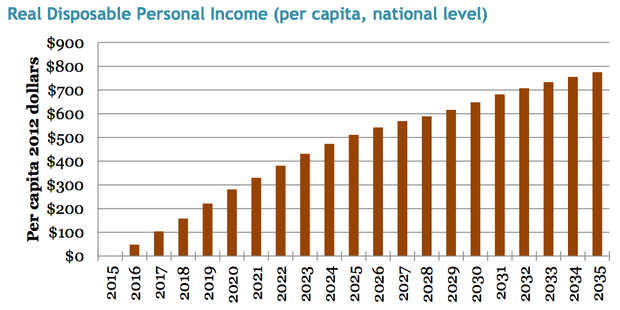
Modeled change in real disposable personal income in the US resulting from the CCL rising revenue-neutral carbon tax. Illustration: Regional Economic Models, Inc.

In short, failing to implement climate policies will certainly slow economic growth, especially in hot, red, southern states. A carbon tax, if crafted smartly, could modestly spur economic growth. Blind opposition to carbon taxes is simply bad for the economy and especially bad for Trump voters.

It’s worse for poorer countries

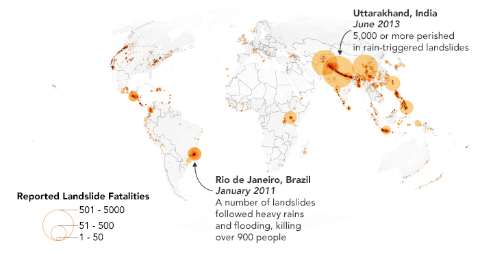
While the Federal Reserve paper focused on the US economy, developing countries will be made much worse off by climate change. Many third world countries are located closer to the equator, where temperatures are already hotter than the temperature sweet spot identified in the 2015 Nature study. A new paperpublished last week in Science Advances also found that these poorer tropical countries will experience bigger temperature swings in a hotter world. Because of this combination of hot temperatures with bigger swings in countries with fewer resources available to adapt, these poorer nations are the most vulnerable to climate change impacts.

This is a key moral and ethical dilemma posed by global warming: as an important 2011 study concluded, the countries that have contributed the least to the problem are the most vulnerable to its consequences. Meanwhile, wealthy countries are already lagging behind their promised financial aid to help poor countries deal with climate change.

Click here to read the rest

from Skeptical Science https://ift.tt/2JWWzFJ

A working paper recently published by the Federal Reserve Bank of Richmond concludes that global warming could significantly slow economic growth in the US.

Specifically, rising summertime temperatures in the hottest states will curb economic growth. And the states with the hottest summertime temperatures are all located in the South: Florida, Louisiana, Texas, Mississippi, Oklahoma, Alabama, Georgia, South Carolina, Arkansas, and Arizona. All of these states voted for Donald Trump in 2016.

This paper is consistent with a 2015 Nature study that found an optimal temperature range for economic activity. Economies thrive in regions with an average temperature of around 14°C (57°F). Developed countries like the US, Japan, and much of Europe happen to be near that ideal temperature, but continued global warming will shift their climates away from the sweet spot and slow economic growth. The question is, by how much?

The new working paper concludes that if we meet the Paris target of staying below 2°C global warming, US economic growth will only slow by about 5 to 10%. On our current path, including climate policies implemented to date (which would lead to 3–3.5°C global warming by 2100), US economic growth would slow by about 10 to 20%. In a higher carbon pollution scenario (4°C global warming by 2100), US economic growth would slow by about 12 to 25% due to hotter temperatures alone.

Republicans have this totally wrong

House Majority Whip Steve Scalise, who represents Louisiana (the second-hottest state), recently introduced a new anti-carbon tax House Resolution. Scalise introduced similar Resolutions in 2013 with 155 co-sponsors (154 Republicans and 1 Democrat) and in 2015 with 82 co-sponsors (all Republicans). The latest version currently only has one co-sponsor, but more will undoubtedly sign on. All three versions of the Resolution include text claiming, “a carbon tax will lead to less economic growth.”

As the economics research shows, failing to curb global warming will certainly lead to less economic growth. Climate policies could hamper economic growth, but legislation can be crafted to address that concern.

For example, as Citizens’ Climate Lobby notes in its point-by-point response to the Scalise Resolution, an economic analysis of the group’s proposed revenue-neutral carbon tax policy found that it would modestly spur economic growth(increasing national GDP by $80 to 90bn per year). With this particular policy, 100% of the carbon tax revenue is returned equally to households, and for a majority of Americans, this more than offsets their increased costs. As a result, real disposable income rises, and Americans spend that money, spurring economic growth.

Modeled change in real disposable personal income in the US resulting from the CCL rising revenue-neutral carbon tax. Illustration: Regional Economic Models, Inc.

In short, failing to implement climate policies will certainly slow economic growth, especially in hot, red, southern states. A carbon tax, if crafted smartly, could modestly spur economic growth. Blind opposition to carbon taxes is simply bad for the economy and especially bad for Trump voters.

It’s worse for poorer countries

While the Federal Reserve paper focused on the US economy, developing countries will be made much worse off by climate change. Many third world countries are located closer to the equator, where temperatures are already hotter than the temperature sweet spot identified in the 2015 Nature study. A new paperpublished last week in Science Advances also found that these poorer tropical countries will experience bigger temperature swings in a hotter world. Because of this combination of hot temperatures with bigger swings in countries with fewer resources available to adapt, these poorer nations are the most vulnerable to climate change impacts.

This is a key moral and ethical dilemma posed by global warming: as an important 2011 study concluded, the countries that have contributed the least to the problem are the most vulnerable to its consequences. Meanwhile, wealthy countries are already lagging behind their promised financial aid to help poor countries deal with climate change.

Click here to read the rest

from Skeptical Science https://ift.tt/2JWWzFJ

Bonding over bones, stones and beads

By Carol Clark

"I've really been into bones since I was little. I don't know why," says Emory University senior Alexandra Davis, an anthropology major. "Not fresh bodies, though. No soft tissues or blood. Just bones."

In fact, Davis loves bones so much that she was willing to spend seven weeks in Malawi with Emory anthropologist Jessica Thompson and four more of her students last summer, excavating bones and other artifacts in ancient hunter-gatherer sites, assisted by a team of locals.

Thompson will return to Malawi in July with another team of students to continue excavation of two sites that were started last summer. "We want to get into the deeper layers, because in both cases we did not come close to reaching the bottom of the sites," Thompson says. "Then, we want to find out how old they are."

Read more about the project.

Related:
Malawi yields oldest-known DNA from Africa
Have skull drill, will travel

from eScienceCommons https://ift.tt/2rpzDbs

By Carol Clark

"I've really been into bones since I was little. I don't know why," says Emory University senior Alexandra Davis, an anthropology major. "Not fresh bodies, though. No soft tissues or blood. Just bones."

In fact, Davis loves bones so much that she was willing to spend seven weeks in Malawi with Emory anthropologist Jessica Thompson and four more of her students last summer, excavating bones and other artifacts in ancient hunter-gatherer sites, assisted by a team of locals.

Thompson will return to Malawi in July with another team of students to continue excavation of two sites that were started last summer. "We want to get into the deeper layers, because in both cases we did not come close to reaching the bottom of the sites," Thompson says. "Then, we want to find out how old they are."

Read more about the project.

Related:
Malawi yields oldest-known DNA from Africa
Have skull drill, will travel

from eScienceCommons https://ift.tt/2rpzDbs

MD studies of simple pericyclic reactions

At the recent ACS meeting in New Orleans, Ken Houk spoke at the Dreyfus award session in honor of Michele Parrinello. Ken’s talk included discussion of some recent molecular dynamics studies of pericyclic reactions. Because of their similarities in approaches and observations, I will discuss three recent papers from his group (which Ken discussed in New Orleans) in this post.

The Cope rearrangement, a fundamental organic reaction, has been studied extensively by computational means (see Chapter 4.2 of my book). Mackey, Yang, and Houk examine the degenerate Cope rearrangement of 1,5-hexadiene with molecular dynamics at the (U)B3LYP/6-31G(d) level.¹ They examined 230 trajectories, and find that of the 95% of them that are reactive, 94% are trajectories that directly cross through the transition zone. By this, Houk means that the time gap between the breaking and forming C-C bonds is less than 60 fs, the time for one C-C bond vibration. The average time in the transition zone is 35 fs. This can be thought of as “dynamically concerted”. For the other few trajectories, a transient diradical with lifetime of about 100 fs is found.

The dimerization of cyclopentadiene finds the two [4+2] pathways merging into a single bispericylic transition state. ² Only a small minority (13%) of the trajectories sample the region about the Cope rearrangement that interconverts the two mirror image dimers. These trajectories average about 60 fs in this space, which comes from the time separation between the formation of the two new C-C bonds. The majority of the trajectories quickly pass through the dimerization transition zone in about 18 fs, and avoid the Cope TS region entirely. These paths can be thought of as “dynamically concerted”, while the other set of trajectories are “dynamically stepwise”. It should be noted however that the value of S² in the Cope transition zone are zero and so no radicals are being formed.

Finally, Yang, Dong, Yu, Yu, Li, Jamieson, and Houk examined 15 different reactions that involve ambimodal (i.e. bispericyclic) transition states.³ They find a strong correlation between the differences in the bond lengths of the two possible new bond vs. their product distribution. So for example, in the reaction shown in Scheme 1, bond a is the one farthest along to forming. Bond b is slightly shorter than bond c. Which of these two is formed next is dependent on the dynamics, and it turns out the P_ab is formed from 73% of the trajectories while P_ac is formed only 23% of the time. This trend is seen across the 15 reaction, namely the shorter of bond b or c in the transition state leads to the larger product formation. When competing reactions involve bonds with differing elements, then a correlation can be found with bond order instead of with bond length.

Scheme 1

References

1) Mackey, J. L.; Yang, Z.; Houk, K. N., "Dynamically concerted and stepwise trajectories of the Cope rearrangement of 1,5-hexadiene." Chem. Phys. Lett. 2017, 683, 253-257, DOI: 10.1016/j.cplett.2017.03.011.

2) Yang, Z.; Zou, L.; Yu, Y.; Liu, F.; Dong, X.; Houk, K. N., "Molecular dynamics of the two-stage mechanism of cyclopentadiene dimerization: concerted or stepwise?" Chem. Phys. 2018, in press, DOI: 10.1016/j.chemphys.2018.02.020.

3) Yang, Z.; Dong, X.; Yu, Y.; Yu, P.; Li, Y.; Jamieson, C.; Houk, K. N., "Relationships between Product Ratios in Ambimodal Pericyclic Reactions and Bond Lengths in Transition Structures." J. Am. Chem. Soc. 2018, 140, 3061-3067, DOI: 10.1021/jacs.7b13562.

from Computational Organic Chemistry https://ift.tt/2HZJOJM

At the recent ACS meeting in New Orleans, Ken Houk spoke at the Dreyfus award session in honor of Michele Parrinello. Ken’s talk included discussion of some recent molecular dynamics studies of pericyclic reactions. Because of their similarities in approaches and observations, I will discuss three recent papers from his group (which Ken discussed in New Orleans) in this post.

The Cope rearrangement, a fundamental organic reaction, has been studied extensively by computational means (see Chapter 4.2 of my book). Mackey, Yang, and Houk examine the degenerate Cope rearrangement of 1,5-hexadiene with molecular dynamics at the (U)B3LYP/6-31G(d) level.¹ They examined 230 trajectories, and find that of the 95% of them that are reactive, 94% are trajectories that directly cross through the transition zone. By this, Houk means that the time gap between the breaking and forming C-C bonds is less than 60 fs, the time for one C-C bond vibration. The average time in the transition zone is 35 fs. This can be thought of as “dynamically concerted”. For the other few trajectories, a transient diradical with lifetime of about 100 fs is found.

The dimerization of cyclopentadiene finds the two [4+2] pathways merging into a single bispericylic transition state. ² Only a small minority (13%) of the trajectories sample the region about the Cope rearrangement that interconverts the two mirror image dimers. These trajectories average about 60 fs in this space, which comes from the time separation between the formation of the two new C-C bonds. The majority of the trajectories quickly pass through the dimerization transition zone in about 18 fs, and avoid the Cope TS region entirely. These paths can be thought of as “dynamically concerted”, while the other set of trajectories are “dynamically stepwise”. It should be noted however that the value of S² in the Cope transition zone are zero and so no radicals are being formed.

Finally, Yang, Dong, Yu, Yu, Li, Jamieson, and Houk examined 15 different reactions that involve ambimodal (i.e. bispericyclic) transition states.³ They find a strong correlation between the differences in the bond lengths of the two possible new bond vs. their product distribution. So for example, in the reaction shown in Scheme 1, bond a is the one farthest along to forming. Bond b is slightly shorter than bond c. Which of these two is formed next is dependent on the dynamics, and it turns out the P_ab is formed from 73% of the trajectories while P_ac is formed only 23% of the time. This trend is seen across the 15 reaction, namely the shorter of bond b or c in the transition state leads to the larger product formation. When competing reactions involve bonds with differing elements, then a correlation can be found with bond order instead of with bond length.

Scheme 1

References

1) Mackey, J. L.; Yang, Z.; Houk, K. N., "Dynamically concerted and stepwise trajectories of the Cope rearrangement of 1,5-hexadiene." Chem. Phys. Lett. 2017, 683, 253-257, DOI: 10.1016/j.cplett.2017.03.011.

2) Yang, Z.; Zou, L.; Yu, Y.; Liu, F.; Dong, X.; Houk, K. N., "Molecular dynamics of the two-stage mechanism of cyclopentadiene dimerization: concerted or stepwise?" Chem. Phys. 2018, in press, DOI: 10.1016/j.chemphys.2018.02.020.

3) Yang, Z.; Dong, X.; Yu, Y.; Yu, P.; Li, Y.; Jamieson, C.; Houk, K. N., "Relationships between Product Ratios in Ambimodal Pericyclic Reactions and Bond Lengths in Transition Structures." J. Am. Chem. Soc. 2018, 140, 3061-3067, DOI: 10.1021/jacs.7b13562.

from Computational Organic Chemistry https://ift.tt/2HZJOJM

Why can’t I find the Milky Way in May?

Milky Way over at Goblin Valley State Park, Utah, by Max Moorman Photography. Read more about this photo. Max acquired this photo in the month of June, when the Milky Way returns to easy viewing in the evening sky.

If you’re in the Northern Hemisphere this month, searching for the starlit band of the Milky Way during the evening hours, you won’t find it. That’s because, on May evenings, the plane of the Milky Way lies in nearly the same plane as that of our horizon as viewed from the northern part of Earth’s globe. The starlit trail doesn’t across the dome of your sky after sunset in May. Instead, it lies nearly flat around your horizon on May evenings.

Want specifics? Here you go. The galactic disk rims the horizon as seen from about 30 degrees North latitude – the latitude of Jacksonville, Florida – Cairo in Egypt – or Chengdu in China.

North of this latitude, the galactic disk tilts a bit upward of the northern horizon during the evening hours in May.

South of 30 degrees north latitude, the galactic disk tilts above the southern horizon. Keep going into Earth’s Southern Hemisphere … and you’ll have a reasonably good view of the Milky Way in the south on May evenings.

It’s all about our view of the sky – from various parts of Earth – as we orbit the sun. Also, although it’s true that the Milky Way galaxy entirely surrounds us in space, the disk of our Milky Way is flat, like a pancake. The illustration below is an all-sky plot of the 25,000 brightest, whitest stars in the Milky Way. It shows how these stars are concentrated along the flat disk of the Milky Way, as seen in our sky:

This illustration of the brightest stars in the Milky Way - as seen in our sky - shows our limited, inside view of our own galaxy. The large, dark patch near the middle of the picture is due to nearby dark nebulae, or clouds of gas and dust, which obscure the stars. Image via altasoftheuniverse.com.

Because the Milky Way rims the horizon in every direction at nightfall and early evening, we can’t see this roadway of stars until later at night. Then … whoa! Beautiful. When will you see the Milky Way again?

Like the sun, the stars rise in the east and set in the west, due to Earth’s rotation or spin on its axis. So you can see the Milky Way tonight if you stay up until late night – say, around midnight in early May, or a couple of hours earlier by June.

Or you can see the Milky Way earlier at night still, as the weeks and months pass, and Earth continues on in its orbit around the sun. As we orbit the sun, our evening sky points out toward an ever-shifting panorama of the galaxy. By June, if you’re standing outside in a rural location on a dark night, you might see the starlit trail of the Milky Way ascending in your eastern sky.

By July or August, the Milky Way will be higher up still in the evening. In fact, August is generally considered the best month for Milky Way viewing. From our hemisphere, the galaxy stretches across the sky on August evenings. The center of the galaxy – where the starlit trail of the Milky Way broadens into a wide boulevard of stars – is visible in the south (for us Northern Hemisphere viewers) in August. From the Southern Hemisphere in August, the view is even better. The center of the Milky Way is closer to overhead in August, from the southerly part of Earth’s globe.

It’ll be beautiful. Just wait.

Enjoying EarthSky so far? Sign up for our free daily newsletter today!

Starlit band of the Milky Way. Photo by Larry Landolfi via NASA.

Bottom line: Assuming you’re in the Northern Hemisphere, the plane of the Milky Way is as parallel to your horizon as it can be, at nightfall and early evening in the month of May. But if you stay up until around midnight, you’ll begin to see the starlit band of the Milky Way ascending in the eastern sky.

EarthSky astronomy kits are perfect for beginners. Order today from the EarthSky store

Donate: Your support means the world to us

from EarthSky https://ift.tt/2rreBs3

Milky Way over at Goblin Valley State Park, Utah, by Max Moorman Photography. Read more about this photo. Max acquired this photo in the month of June, when the Milky Way returns to easy viewing in the evening sky.

If you’re in the Northern Hemisphere this month, searching for the starlit band of the Milky Way during the evening hours, you won’t find it. That’s because, on May evenings, the plane of the Milky Way lies in nearly the same plane as that of our horizon as viewed from the northern part of Earth’s globe. The starlit trail doesn’t across the dome of your sky after sunset in May. Instead, it lies nearly flat around your horizon on May evenings.

Want specifics? Here you go. The galactic disk rims the horizon as seen from about 30 degrees North latitude – the latitude of Jacksonville, Florida – Cairo in Egypt – or Chengdu in China.

North of this latitude, the galactic disk tilts a bit upward of the northern horizon during the evening hours in May.

South of 30 degrees north latitude, the galactic disk tilts above the southern horizon. Keep going into Earth’s Southern Hemisphere … and you’ll have a reasonably good view of the Milky Way in the south on May evenings.

It’s all about our view of the sky – from various parts of Earth – as we orbit the sun. Also, although it’s true that the Milky Way galaxy entirely surrounds us in space, the disk of our Milky Way is flat, like a pancake. The illustration below is an all-sky plot of the 25,000 brightest, whitest stars in the Milky Way. It shows how these stars are concentrated along the flat disk of the Milky Way, as seen in our sky:

This illustration of the brightest stars in the Milky Way - as seen in our sky - shows our limited, inside view of our own galaxy. The large, dark patch near the middle of the picture is due to nearby dark nebulae, or clouds of gas and dust, which obscure the stars. Image via altasoftheuniverse.com.

Because the Milky Way rims the horizon in every direction at nightfall and early evening, we can’t see this roadway of stars until later at night. Then … whoa! Beautiful. When will you see the Milky Way again?

Like the sun, the stars rise in the east and set in the west, due to Earth’s rotation or spin on its axis. So you can see the Milky Way tonight if you stay up until late night – say, around midnight in early May, or a couple of hours earlier by June.

Or you can see the Milky Way earlier at night still, as the weeks and months pass, and Earth continues on in its orbit around the sun. As we orbit the sun, our evening sky points out toward an ever-shifting panorama of the galaxy. By June, if you’re standing outside in a rural location on a dark night, you might see the starlit trail of the Milky Way ascending in your eastern sky.

By July or August, the Milky Way will be higher up still in the evening. In fact, August is generally considered the best month for Milky Way viewing. From our hemisphere, the galaxy stretches across the sky on August evenings. The center of the galaxy – where the starlit trail of the Milky Way broadens into a wide boulevard of stars – is visible in the south (for us Northern Hemisphere viewers) in August. From the Southern Hemisphere in August, the view is even better. The center of the Milky Way is closer to overhead in August, from the southerly part of Earth’s globe.

It’ll be beautiful. Just wait.

Enjoying EarthSky so far? Sign up for our free daily newsletter today!

Starlit band of the Milky Way. Photo by Larry Landolfi via NASA.

Bottom line: Assuming you’re in the Northern Hemisphere, the plane of the Milky Way is as parallel to your horizon as it can be, at nightfall and early evening in the month of May. But if you stay up until around midnight, you’ll begin to see the starlit band of the Milky Way ascending in the eastern sky.

EarthSky astronomy kits are perfect for beginners. Order today from the EarthSky store

Donate: Your support means the world to us

from EarthSky https://ift.tt/2rreBs3

New science from Jupiter

NASA’s Juno mission launched on August 5, 2011, traveled 1.74 billion miles (2.8 billion km) and entered Jupiter’s orbit on July 4, 2016.

This new NASA ScienceCast video rounds up some of Juno’s coolest finds.

Juno’s mission is to measure Jupiter’s composition, gravity field, magnetic field, and polar magnetosphere. It’s also searching for clues about how the planet formed, including whether it has a rocky core; how much water there is within the deep atmosphere; and Jupiter’s deep winds, which can reach speeds up to 384 miles per hour (618 km per hour).

Bottom line: NASA video describes the newest science from the Juno mission to Jupiter.

Read more from NASA

from EarthSky https://ift.tt/2jC7g5y

NASA’s Juno mission launched on August 5, 2011, traveled 1.74 billion miles (2.8 billion km) and entered Jupiter’s orbit on July 4, 2016.

This new NASA ScienceCast video rounds up some of Juno’s coolest finds.

Juno’s mission is to measure Jupiter’s composition, gravity field, magnetic field, and polar magnetosphere. It’s also searching for clues about how the planet formed, including whether it has a rocky core; how much water there is within the deep atmosphere; and Jupiter’s deep winds, which can reach speeds up to 384 miles per hour (618 km per hour).

Bottom line: NASA video describes the newest science from the Juno mission to Jupiter.

Read more from NASA

from EarthSky https://ift.tt/2jC7g5y

Help NASA create the world’s largest landslide database

Landslide of June, 1, 2007, on a mountain near Canmore in Alberta, Canada, via Flickr user Sheri Teris/ NASA.

Originally posted April 18, 2018, by Kasha Patel at NASA Earth Observatory

Landslides cause thousands of deaths and billions of dollars in property damage each year. Surprisingly, very few centralized global landslide databases exist, especially those that are publicly available.

Now NASA scientists are working to fill the gap—and they want your help collecting information. In March 2018, NASA scientist Dalia Kirschbaum and several colleagues launched a citizen science project that will make it possible to report landslides you have witnessed, heard about in the news, or found on an online database. All you need to do is log into the Landslide Reporter portal and report the time, location, and date of the landslide—as well as your source of information. You are also encouraged to submit additional details, such as the size of the landslide and what triggered it. And if you have photos, you can upload them.

Research scientist Dalia Kirshbaum wants to hear from you about landslides at the Landslide Reporter portal.

Kirschbaum’s team will review each entry and submit credible reports to the Cooperative Open Online Landslide Repository (COOLR) — which they hope will eventually be the largest global online landslide catalog available.

Report landslides and upload photos here

Landslide Reporter is designed to improve the quantity and quality of data in COOLR. Currently, COOLR contains NASA’s Global Landslide Catalog, which includes more than 11,000 reports on landslides, debris flows, and rock avalanches. Since the current catalog is based mainly on information from English language news reports and journalists tend to cover only large and deadly landslides in densely populated areas, many landslides never make it into the database.

Landslide Reporter should help change this because it makes it possible for people to submit reports, including first-hand accounts, from anywhere in the world.

Kirschbaum plans to use this database to improve the algorithm for her team’s landslide prediction model. The model, known as the Landslide Hazard Assessment for Situational Awareness (LHASA) model, analyzes rainfall and land characteristics in an area that might make a landslide more susceptible. The model produces forecasts of potential landslide activity every 30 minutes. In some cases, however, the model predicts more or less potential activity. Kirschbaum said:

With more ground data to validate the model, we can create a better tool for improving situational awareness and research for this pervasive hazard. We could better anticipate and forecast where landslides may impact populations.

Check out posts by Caroline Juang on Discover magazine’s citizen science blog and by David Petley on American Geophysical Union’s Landslide Blog to find out more. You can also follow the project on Twitter (@LandslideReport) and at Landslide Reporter on Facebook.

This map shows 2,085 landslides with fatalities as reported in the Global Landslide Catalog, which is currently included in the Cooperative Open Online Landslide Repository (COOLR). NASA Earth Observatory images by Joshua Stevens, using landslide susceptibility data provided by Thomas Stanley and Dalia Kirschbaum (NASA/GSFC).

Bottom line: NASA researchers led by Dalia Kirshbaum have launched a citizen science project requesting your reports and photos of landslides. Report landslides and upload photos here.

from EarthSky https://ift.tt/2I0Owak

Landslide of June, 1, 2007, on a mountain near Canmore in Alberta, Canada, via Flickr user Sheri Teris/ NASA.

Originally posted April 18, 2018, by Kasha Patel at NASA Earth Observatory

Landslides cause thousands of deaths and billions of dollars in property damage each year. Surprisingly, very few centralized global landslide databases exist, especially those that are publicly available.

Now NASA scientists are working to fill the gap—and they want your help collecting information. In March 2018, NASA scientist Dalia Kirschbaum and several colleagues launched a citizen science project that will make it possible to report landslides you have witnessed, heard about in the news, or found on an online database. All you need to do is log into the Landslide Reporter portal and report the time, location, and date of the landslide—as well as your source of information. You are also encouraged to submit additional details, such as the size of the landslide and what triggered it. And if you have photos, you can upload them.

Research scientist Dalia Kirshbaum wants to hear from you about landslides at the Landslide Reporter portal.

Kirschbaum’s team will review each entry and submit credible reports to the Cooperative Open Online Landslide Repository (COOLR) — which they hope will eventually be the largest global online landslide catalog available.

Report landslides and upload photos here

Landslide Reporter is designed to improve the quantity and quality of data in COOLR. Currently, COOLR contains NASA’s Global Landslide Catalog, which includes more than 11,000 reports on landslides, debris flows, and rock avalanches. Since the current catalog is based mainly on information from English language news reports and journalists tend to cover only large and deadly landslides in densely populated areas, many landslides never make it into the database.

Landslide Reporter should help change this because it makes it possible for people to submit reports, including first-hand accounts, from anywhere in the world.

Kirschbaum plans to use this database to improve the algorithm for her team’s landslide prediction model. The model, known as the Landslide Hazard Assessment for Situational Awareness (LHASA) model, analyzes rainfall and land characteristics in an area that might make a landslide more susceptible. The model produces forecasts of potential landslide activity every 30 minutes. In some cases, however, the model predicts more or less potential activity. Kirschbaum said:

With more ground data to validate the model, we can create a better tool for improving situational awareness and research for this pervasive hazard. We could better anticipate and forecast where landslides may impact populations.

Check out posts by Caroline Juang on Discover magazine’s citizen science blog and by David Petley on American Geophysical Union’s Landslide Blog to find out more. You can also follow the project on Twitter (@LandslideReport) and at Landslide Reporter on Facebook.

This map shows 2,085 landslides with fatalities as reported in the Global Landslide Catalog, which is currently included in the Cooperative Open Online Landslide Repository (COOLR). NASA Earth Observatory images by Joshua Stevens, using landslide susceptibility data provided by Thomas Stanley and Dalia Kirschbaum (NASA/GSFC).

Bottom line: NASA researchers led by Dalia Kirshbaum have launched a citizen science project requesting your reports and photos of landslides. Report landslides and upload photos here.

from EarthSky https://ift.tt/2I0Owak

What causes landslides?

A view from a Washington Army National Guard helicopter showing the aftermath of the March 22, 2014, mudslide in Oso, Washington, more than a week after it occurred. Image via DVIDS.

The terms landslide or mudslide refer to the downward movement of large masses of rocks, soil, mud and organic debris. Areas with steep slopes, for example mountainous regions, are particularly susceptible to landslide hazards. Most landslides are caused by multiple factors that act together to destabilize the slope.

The primary cause of a landslide is the influence of gravity acting on weakened materials that make up a sloping area of land. While some landslides occur slowly over time (e.g., land movement on the order of a few meters per month), the most destructive ones happen suddenly after a triggering event such as heavy rainfall or an earthquake.

That was the case for the last extremely deadly mudslide in the continental U.S., the 2014 Oso mudslide, which took 43 lives and destroyed 49 homes and other structures. A portion of an unstable hill collapsed, sending mud and debris to the south across the North Fork of the Stillaguamish River, engulfing a rural neighborhood. Prior to the slide, the Oso area – which is about 55 miles northeast of Seattle – had had heavy rainfall during the previous 45 days, up to 261 percent of normal, by some sources.

The Oso, Washington, mudslide as viewed from the air on March 24, 2014. Photo by Ted S. Warren/Concord Monitor. Experts said that the primary reason for the Oso mudslide was rain.

Water can trigger landslides and mudslides because it alters the pressure within the slope, which leads to slope instability. Consequently, the heavy water-laden slope materials (soil, rock, etc.) will succumb to the forces of gravity. Excessive water is thought to be one of the most common triggers for landslides.

Other factors that weaken slope materials also contribute to the occurrence of landslides. These factors include both natural events such as geological weathering and erosion and human-related activities such as deforestation and changes made to the flow of groundwater. Destruction of vegetation by droughts, fires, and logging has been associated with increased risk for landslides.

Aerial view of the Oso area shortly after the March 22, 2014, mudslide. The slide covered about a 1-square-mile (2.6-square-km) area. Image via U.S. Navy/Wikimedia Commons.

Landslides are classified according to the type of material that falls and how that material moves downslope. For example, there are rock falls, mudslides, and debris flows. All of these terms represent a type of landslide.

One particularly destructive type of landslide is known as a lahar. Lahars are volcanic mud flows or debris flows that are capable of traveling at very fast speeds down the slope of a volcano.

The Landslide Handbook – A Guide to Understanding Landslides is a great resource from the U.S. Geological Survey for those who want to learn more about landslides.

A lahar resulting from a 1982 eruption of the Galunggung volcano in Indonesia. Image via Robin Holcomb, U.S. Geological Survey.

Bottom line: Landslides are mainly caused by gravity acting on weakened rocks and soil that make up a sloping area of land. Both natural and human-related activities can increase the risk for landslides. Water from heavy rainfall is a frequent trigger for landslides.

Before and after images of enormous landslide in Alaska

from EarthSky https://ift.tt/25SrMQY

A view from a Washington Army National Guard helicopter showing the aftermath of the March 22, 2014, mudslide in Oso, Washington, more than a week after it occurred. Image via DVIDS.

The terms landslide or mudslide refer to the downward movement of large masses of rocks, soil, mud and organic debris. Areas with steep slopes, for example mountainous regions, are particularly susceptible to landslide hazards. Most landslides are caused by multiple factors that act together to destabilize the slope.

The primary cause of a landslide is the influence of gravity acting on weakened materials that make up a sloping area of land. While some landslides occur slowly over time (e.g., land movement on the order of a few meters per month), the most destructive ones happen suddenly after a triggering event such as heavy rainfall or an earthquake.

That was the case for the last extremely deadly mudslide in the continental U.S., the 2014 Oso mudslide, which took 43 lives and destroyed 49 homes and other structures. A portion of an unstable hill collapsed, sending mud and debris to the south across the North Fork of the Stillaguamish River, engulfing a rural neighborhood. Prior to the slide, the Oso area – which is about 55 miles northeast of Seattle – had had heavy rainfall during the previous 45 days, up to 261 percent of normal, by some sources.

The Oso, Washington, mudslide as viewed from the air on March 24, 2014. Photo by Ted S. Warren/Concord Monitor. Experts said that the primary reason for the Oso mudslide was rain.

Water can trigger landslides and mudslides because it alters the pressure within the slope, which leads to slope instability. Consequently, the heavy water-laden slope materials (soil, rock, etc.) will succumb to the forces of gravity. Excessive water is thought to be one of the most common triggers for landslides.

Other factors that weaken slope materials also contribute to the occurrence of landslides. These factors include both natural events such as geological weathering and erosion and human-related activities such as deforestation and changes made to the flow of groundwater. Destruction of vegetation by droughts, fires, and logging has been associated with increased risk for landslides.

Aerial view of the Oso area shortly after the March 22, 2014, mudslide. The slide covered about a 1-square-mile (2.6-square-km) area. Image via U.S. Navy/Wikimedia Commons.

Landslides are classified according to the type of material that falls and how that material moves downslope. For example, there are rock falls, mudslides, and debris flows. All of these terms represent a type of landslide.

One particularly destructive type of landslide is known as a lahar. Lahars are volcanic mud flows or debris flows that are capable of traveling at very fast speeds down the slope of a volcano.

The Landslide Handbook – A Guide to Understanding Landslides is a great resource from the U.S. Geological Survey for those who want to learn more about landslides.

A lahar resulting from a 1982 eruption of the Galunggung volcano in Indonesia. Image via Robin Holcomb, U.S. Geological Survey.

Bottom line: Landslides are mainly caused by gravity acting on weakened rocks and soil that make up a sloping area of land. Both natural and human-related activities can increase the risk for landslides. Water from heavy rainfall is a frequent trigger for landslides.

Before and after images of enormous landslide in Alaska

from EarthSky https://ift.tt/25SrMQY