Analysis reveals tiny dino with rainbow feathers

Caihong juji is a newly described, bird-like dinosaur with an iridescent, rainbow crest. It lived in China about 161 million years ago, and may have used its impressive feathers to attract mates. Illustration by Velizar Simeonovski, The Field Museum, via UT Austin Jackson School of Geosciences.

A team of researchers have conducted a study of the remains of chicken-sized dinosaur that lived in China about 161 million years ago, during the Jurassic period. Their analysis of the exquisitely-preserved fossil, published January 15, 2018 in the journal Nature Communications, suggests that the small dinosaur had a shaggy ruff of iridescent rainbow feathers.

The scientists think the dinosaur – named Caihong juji, “rainbow with the big crest” in Mandarin — used its flashy neck feathers and a bony crest on its snout to attract mates.

Julia Clarke, a professor in the Department of Geological Sciences at the Univeristy of Texas Jackson School of Geosciences, helped describe the new species. She said in a statement:

Iridescent coloration is well known to be linked to sexual selection and signaling, and we report its earliest evidence in dinosaurs.

The slab of rock containing the dinosaur fossil included a nearly complete skeleton (brown) as well as feather impressions (black). Image via Hu, et al., 2018.

The dinosaur is interesting because it has features that are both ancient and modern, said co-author Xing Xu, a professor at the Chinese Academy of Sciences. The bony crest is a feature usually seen in dinosaurs from earlier eras, while its neck feathers show evidence of melanosomes – microscopic, wide, pigment-containing packages – that may represent the first known occurrence of iridescence similar to that found in many of today’s hummingbirds.

A farmer discovered the slab of rock containing the dinosaur fossil in northern China’s Hebei Province in 2014. The rock contained a nearly complete skeleton surrounded by impressions made by feathers. The impressions preserved the shape of the melanosomes. The researchers compared the melanosome impressions to melanosomes found in living birds and found that they most closely resembled those in the iridescent, rainbow feathers of hummingbirds.

The long and narrow dinosaur skull is similar to a Velociraptor’s, a shape that is unique among bird-like dinosaurs. The scale bar is 1 centimeter long. Image via Hu, et al., 2018.

Caihong is also the earliest known dinosaur with asymmetrical feathers, the feather type found on the wingtips of modern birds that helps control flight, said the researchers. But unlike birds today, Caihong’s asymmetrical feathers were on its tail, not its wings — a finding that suggests that early birds may have had a different steering or flight style.

Caihong stands out from the other small, bird-like dinosaurs that lived in China during the Jurassic, the researchers say. While the other dinosaurs had triangular skulls and longer forearm bones than today’s birds, Caihong had a long and narrow skull, and unlike many of these other dinosaurs, its short forelimbs show proportions more like modern birds. Clarke said:

This combination of traits is unusual. It has a rather velociraptor-looking low and long skull with this fully feathered, shaggy kind of plumage and a big fan tail. It is really cool… or maybe creepy looking depending on your perspective.

Bottom line: Researchers have described a small dinosaur with rainbow feathers that lived in China about 161 million years ago.

Read more from the University of Texas/Austin

from EarthSky http://ift.tt/2rH2RVK

Caihong juji is a newly described, bird-like dinosaur with an iridescent, rainbow crest. It lived in China about 161 million years ago, and may have used its impressive feathers to attract mates. Illustration by Velizar Simeonovski, The Field Museum, via UT Austin Jackson School of Geosciences.

A team of researchers have conducted a study of the remains of chicken-sized dinosaur that lived in China about 161 million years ago, during the Jurassic period. Their analysis of the exquisitely-preserved fossil, published January 15, 2018 in the journal Nature Communications, suggests that the small dinosaur had a shaggy ruff of iridescent rainbow feathers.

The scientists think the dinosaur – named Caihong juji, “rainbow with the big crest” in Mandarin — used its flashy neck feathers and a bony crest on its snout to attract mates.

Julia Clarke, a professor in the Department of Geological Sciences at the Univeristy of Texas Jackson School of Geosciences, helped describe the new species. She said in a statement:

Iridescent coloration is well known to be linked to sexual selection and signaling, and we report its earliest evidence in dinosaurs.

The slab of rock containing the dinosaur fossil included a nearly complete skeleton (brown) as well as feather impressions (black). Image via Hu, et al., 2018.

The dinosaur is interesting because it has features that are both ancient and modern, said co-author Xing Xu, a professor at the Chinese Academy of Sciences. The bony crest is a feature usually seen in dinosaurs from earlier eras, while its neck feathers show evidence of melanosomes – microscopic, wide, pigment-containing packages – that may represent the first known occurrence of iridescence similar to that found in many of today’s hummingbirds.

A farmer discovered the slab of rock containing the dinosaur fossil in northern China’s Hebei Province in 2014. The rock contained a nearly complete skeleton surrounded by impressions made by feathers. The impressions preserved the shape of the melanosomes. The researchers compared the melanosome impressions to melanosomes found in living birds and found that they most closely resembled those in the iridescent, rainbow feathers of hummingbirds.

The long and narrow dinosaur skull is similar to a Velociraptor’s, a shape that is unique among bird-like dinosaurs. The scale bar is 1 centimeter long. Image via Hu, et al., 2018.

Caihong is also the earliest known dinosaur with asymmetrical feathers, the feather type found on the wingtips of modern birds that helps control flight, said the researchers. But unlike birds today, Caihong’s asymmetrical feathers were on its tail, not its wings — a finding that suggests that early birds may have had a different steering or flight style.

Caihong stands out from the other small, bird-like dinosaurs that lived in China during the Jurassic, the researchers say. While the other dinosaurs had triangular skulls and longer forearm bones than today’s birds, Caihong had a long and narrow skull, and unlike many of these other dinosaurs, its short forelimbs show proportions more like modern birds. Clarke said:

This combination of traits is unusual. It has a rather velociraptor-looking low and long skull with this fully feathered, shaggy kind of plumage and a big fan tail. It is really cool… or maybe creepy looking depending on your perspective.

Bottom line: Researchers have described a small dinosaur with rainbow feathers that lived in China about 161 million years ago.

Read more from the University of Texas/Austin

from EarthSky http://ift.tt/2rH2RVK

Cartwheel Galaxy

Image via ESA/Hubble & NASA.

There are some standard shapes for galaxies in our universe, including spiral shapes like our Milky Way – elliptical, or football-like shapes – and irregulars. This Hubble Space Telescope image shows a rare breed of galaxy, a ring galaxy, called of the Cartwheel Galaxy. It lies about 500 million light-years away in the direction to the southern constellation Sculptor.

Astronomers first spotted this galaxy in 1941. They say its cartwheel shape is the result of a violent galactic collision. A smaller galaxy passed right through a large disk galaxy and produced shock waves that swept up gas and dust — much like the ripples produced when a stone is dropped into a lake — and sparked regions of intense star formation (colored blue). The outermost ring of the galaxy, which is 1.5 times the size of our Milky Way, marks the shock wave’s leading edge.

This object is one of the most dramatic examples of the small class of ring galaxies.

This image is based on earlier Hubble data of the Cartwheel Galaxy that was reprocessed in 2010, bringing out more detail in the image than seen before.

Read more from NASA

Bottom line: Hubble Space Telescope image of the Cartwheel galaxy.

from EarthSky http://ift.tt/2E7DLlj

Image via ESA/Hubble & NASA.

There are some standard shapes for galaxies in our universe, including spiral shapes like our Milky Way – elliptical, or football-like shapes – and irregulars. This Hubble Space Telescope image shows a rare breed of galaxy, a ring galaxy, called of the Cartwheel Galaxy. It lies about 500 million light-years away in the direction to the southern constellation Sculptor.

Astronomers first spotted this galaxy in 1941. They say its cartwheel shape is the result of a violent galactic collision. A smaller galaxy passed right through a large disk galaxy and produced shock waves that swept up gas and dust — much like the ripples produced when a stone is dropped into a lake — and sparked regions of intense star formation (colored blue). The outermost ring of the galaxy, which is 1.5 times the size of our Milky Way, marks the shock wave’s leading edge.

This object is one of the most dramatic examples of the small class of ring galaxies.

This image is based on earlier Hubble data of the Cartwheel Galaxy that was reprocessed in 2010, bringing out more detail in the image than seen before.

Read more from NASA

Bottom line: Hubble Space Telescope image of the Cartwheel galaxy.

from EarthSky http://ift.tt/2E7DLlj

Hyades star cluster: Face of Taurus

The Hyades. Copyright Jerry Lodriguss/ AstroPix.com Used with permission

With the exception of the Ursa Major Moving Cluster, the Hyades cluster is the closest star cluster to Earth, at a distance of 150 light-years. This cluster is very easy to spot in the night sky, because it has a compact and distinctive shape of the letter V. The bright star Aldebaran is part of the V. Follow the links below to learn more about the Hyades.

How to find the Hyades star cluster.

History and mythology of the Hyades.

Hyades science.

Moon near brightest star in Hyades, Aldebaran, on January 26, 2018

The Hyades star cluster can be found easily on January and February evenings, and is edging toward the western half of the sky by March and April evenings. It has the shape of the letter V. The brightest star in the V in Aldebaran. The small dipper-shaped Pleiades star cluster is nearby.

Here are Orion, the bright star Aldebaran in Taurus, and the Pleiades. Notice the three stars of Orion’s “Belt,” that is, three stars in a short row. Notice that these stars point to Aldebaran.

How to find the Hyades star cluster. The Hyades cluster is easy to find by using Orion’s Belt, a compact and noticeable line of three blue-white stars in the constellation Orion the Hunter. Draw a line westward (generally toward your sunset direction) through the Belt stars, and you will come to the bright reddish star Aldebaran, the Bull’s fiery red eye.

Aldebaran is part of the V-shape formation of stars that represents in the Bull’s face. This V of stars is the Hyades.

Although Aldebaran isn’t a true member of the Hyades star cluster, this bright star is a great guide to this cluster. In fact, Aldebaran is only about 65 light-years distant. The Hyades lies about 2.5 times farther off.

The V-shape figurine of stars (except Aldebaran) highlights the brightest of the Hyades’ few hundred stars. A dozen or more Hyades stars are visible to the unaided eye in a dark country sky, but several dozen of the cluster’s stars can be resolved through binoculars or low power in a telescope. From the northern hemisphere, the Hyades are best seen in the evening sky from around January to April.

The constellation Taurus the Bull is home to another bright star cluster, the Pleiades. The Pleiades cluster is more distant than the Hyades at some 430 light-years away. Both the Hyades and Pleiades are easily visible to the unaided eye. Both are enhanced by viewing with binoculars.

The Hyades – like their half sister the Pleiades – were nymphs of Greek mythology. Image via Greek Mythology Link – by Carlos Parada

History and mythology of the Hyades. According to sky lore, the teary Hyades are the daughters of Atlas and Aethra, who are forever crying for their brother Hyas, who was killed by a lion or a boar. The Hyades are the half sisters to the Pleiades, the daughters of Atlas and Pleione. The gods purposely kept Atlas’ daughters – the Hyades and the Pleaides – out of reach of Orion, giving them a safe haven from his lustful pursuits.

The gods transformed Hyas into the constellation Aquarius, and the lion that killed him into the constellation Leo. The gods placed Aquarius and Leo on opposite sides of the sky for Hyas’ protection. That’s why Aquarius and Leo do not appear in the same sky together. As one constellation sets in the west, the other rises in the east – and vice versa.

A telescope reveals over 100 stars in the Hyades cluster. The bright red star here is Aldebaran. Photo via astronomycafe.net.

Hyades science. Although the Hyades and Pleaides are half sisters in mythology, science finds no close relationship in space between these two star clusters.

Astronomers find that the Pleiades are composed of hot blue-white suns in the heyday of youth, which puts the age of the cluster at about 100 million years. In contrast, the cooler red giant and white dwarf stars found in the Hyades indicate a vastly older cluster over 700 million years old.

Interestingly, astronomers suspect an actual kinship between the Hyades cluster and the Beehive star cluster in the constellation Cancer the Crab. Even though these two star clusters are separated from one another by hundreds of light-years, they are akin in age and travel in a similar direction in space. Astronomers believe these clusters might have originated from the same gaseous nebula some 700 to 800 million years ago.

The three bright stars in a row are Orion’s Belt. They point to the Hyades star cluster. Photo via Unishot/Flickr

View larger. | More detail on the starry sky around the Hyades. Notice that Orion's Belt (lower left) points to the Hyades.

Enjoying EarthSky? Sign up for our free daily newsletter today!

Bottom line: On January evenings, look for a V-shaped pattern of stars. The Hyades star cluster represents the Face of Taurus the Bull. The cluster is easy to spot and beautiful in binoculars.

from EarthSky http://ift.tt/1oyhBs9

The Hyades. Copyright Jerry Lodriguss/ AstroPix.com Used with permission

With the exception of the Ursa Major Moving Cluster, the Hyades cluster is the closest star cluster to Earth, at a distance of 150 light-years. This cluster is very easy to spot in the night sky, because it has a compact and distinctive shape of the letter V. The bright star Aldebaran is part of the V. Follow the links below to learn more about the Hyades.

How to find the Hyades star cluster.

History and mythology of the Hyades.

Hyades science.

Moon near brightest star in Hyades, Aldebaran, on January 26, 2018

The Hyades star cluster can be found easily on January and February evenings, and is edging toward the western half of the sky by March and April evenings. It has the shape of the letter V. The brightest star in the V in Aldebaran. The small dipper-shaped Pleiades star cluster is nearby.

Here are Orion, the bright star Aldebaran in Taurus, and the Pleiades. Notice the three stars of Orion’s “Belt,” that is, three stars in a short row. Notice that these stars point to Aldebaran.

How to find the Hyades star cluster. The Hyades cluster is easy to find by using Orion’s Belt, a compact and noticeable line of three blue-white stars in the constellation Orion the Hunter. Draw a line westward (generally toward your sunset direction) through the Belt stars, and you will come to the bright reddish star Aldebaran, the Bull’s fiery red eye.

Aldebaran is part of the V-shape formation of stars that represents in the Bull’s face. This V of stars is the Hyades.

Although Aldebaran isn’t a true member of the Hyades star cluster, this bright star is a great guide to this cluster. In fact, Aldebaran is only about 65 light-years distant. The Hyades lies about 2.5 times farther off.

The V-shape figurine of stars (except Aldebaran) highlights the brightest of the Hyades’ few hundred stars. A dozen or more Hyades stars are visible to the unaided eye in a dark country sky, but several dozen of the cluster’s stars can be resolved through binoculars or low power in a telescope. From the northern hemisphere, the Hyades are best seen in the evening sky from around January to April.

The constellation Taurus the Bull is home to another bright star cluster, the Pleiades. The Pleiades cluster is more distant than the Hyades at some 430 light-years away. Both the Hyades and Pleiades are easily visible to the unaided eye. Both are enhanced by viewing with binoculars.

The Hyades – like their half sister the Pleiades – were nymphs of Greek mythology. Image via Greek Mythology Link – by Carlos Parada

History and mythology of the Hyades. According to sky lore, the teary Hyades are the daughters of Atlas and Aethra, who are forever crying for their brother Hyas, who was killed by a lion or a boar. The Hyades are the half sisters to the Pleiades, the daughters of Atlas and Pleione. The gods purposely kept Atlas’ daughters – the Hyades and the Pleaides – out of reach of Orion, giving them a safe haven from his lustful pursuits.

The gods transformed Hyas into the constellation Aquarius, and the lion that killed him into the constellation Leo. The gods placed Aquarius and Leo on opposite sides of the sky for Hyas’ protection. That’s why Aquarius and Leo do not appear in the same sky together. As one constellation sets in the west, the other rises in the east – and vice versa.

A telescope reveals over 100 stars in the Hyades cluster. The bright red star here is Aldebaran. Photo via astronomycafe.net.

Hyades science. Although the Hyades and Pleaides are half sisters in mythology, science finds no close relationship in space between these two star clusters.

Astronomers find that the Pleiades are composed of hot blue-white suns in the heyday of youth, which puts the age of the cluster at about 100 million years. In contrast, the cooler red giant and white dwarf stars found in the Hyades indicate a vastly older cluster over 700 million years old.

Interestingly, astronomers suspect an actual kinship between the Hyades cluster and the Beehive star cluster in the constellation Cancer the Crab. Even though these two star clusters are separated from one another by hundreds of light-years, they are akin in age and travel in a similar direction in space. Astronomers believe these clusters might have originated from the same gaseous nebula some 700 to 800 million years ago.

The three bright stars in a row are Orion’s Belt. They point to the Hyades star cluster. Photo via Unishot/Flickr

View larger. | More detail on the starry sky around the Hyades. Notice that Orion's Belt (lower left) points to the Hyades.

Enjoying EarthSky? Sign up for our free daily newsletter today!

Bottom line: On January evenings, look for a V-shaped pattern of stars. The Hyades star cluster represents the Face of Taurus the Bull. The cluster is easy to spot and beautiful in binoculars.

from EarthSky http://ift.tt/1oyhBs9

Moon near former pole star January 26

Tonight – January 26, 2018 – the waxing gibbous moon passes in the vicinity of Aldebaran, an ex-pole star, a famous zodiac star, and the brightest star in the constellation Taurus the Bull.

If you live in northwestern North America, you can watch the moon occult – cover over – Aldebaran for a portion of the night on this date. Aldebaran will disappear behind the moon’s dark side and reappear on its illuminated side. So the disappearance will probably be easier to spot than the reappearance.

Worldwide map of the occultation of Aldebaran via IOTA. Everyplace to the north or above the white arc sees the occultation in a nighttime sky. The turquoise loop in North America depicts where the disappearance is visible but where Aldebaran sets before Aldebaran can reappear. Click here for details.

Click here if you’re in northwestern North America and want to know the occultation times. You must convert Coordinated Universal Time (UTC) to your local time (PST = UTC-8 hours; Alaska = UTC-9 hours). For your convenience, we give the local time that Aldebaran disappears behind the moon’s dark limb for Seattle, Washington (January 27 at 3:13 a.m. local time) and Anchorage, Alaska (January 27 at 1:54 a.m. local time).

The rest of us will see Aldebaran near the moon on this date. It’s a wonderful time to learn to identify this star, even though you might have to squint a bit to see it in the moon’s glare.

Aldebaran is a bright reddish star, a good star to come to know. Did you know that Aldebaran is also a former pole star? It’s true, and it’s a fascinating story.

Many people know that Polaris is the present-day North Star, but few know that Aldebaran reigned as the North Star some 450,000 years ago.

What’s more, Aldebaran appeared several times brighter in the sky then than it does now. Plus – 450,000 years ago – Aldebaran shone very close to the very bright star Capella on the sky’s dome. In that distant past, these two brilliant stars served as a double pole star in the astronomical year -447,890 (447,891 BC).

View larger. | This illustration shows the view from present-day Arizona in 447,000 B.C., when Aldebaran and Capella served as double pole stars. Illustration via Carina Software and Instruments.

At this point, we should probably insert a note about astronomical dating. In ancient times, there was no zero year, so the year AD 1 followed the year 1 BC. However, present-day astronomical calculating is made simpler by equating the astronomical year 0 with the year 1 BC. Thus, the astronomical year -1 corresponds to 2 BC and the astronomical year -2 corresponds to 3 BC. And so on . . .

But back to Aldebaran and Capella as dual pole stars. The identity of the pole star shifts over time, due to the 26,000-year cycle of precession. To read more about that, click into this article about Thuban, another former pole star.

Still, how can it be, you might wonder, that the stars Aldebaran and Capella were once so near each other on the sky’s dome? They’re not especially close together now. Aren’t the stars essentially fixed relative to one another? The answer is that, yes, on the scale of human lifespans, the stars are essentially fixed. But the stars are actually moving through space, in orbit around the center of the galaxy. In our solar system, galaxy and universe … everything is always moving. So the sky looked different hundreds of thousands of years ago than it does today.

So watch for Aldebaran near the moon tonight, and think back to 450,000 years ago, when Aldebaran and Capella teamed up together to serve as Earth’s double north pole star!*

*Source: Page 363 of Mathematical Astronomy Morsels V by Jean Meeus

EarthSky astronomy kits are perfect for beginners. Order today from the EarthSky store

Bottom line: Will you see Aldebaran in the moon’s glare on January 26, 2018? Plus … the story of Aldebaran when it was part of a double pole star.

from EarthSky http://ift.tt/2iRooD8

Tonight – January 26, 2018 – the waxing gibbous moon passes in the vicinity of Aldebaran, an ex-pole star, a famous zodiac star, and the brightest star in the constellation Taurus the Bull.

If you live in northwestern North America, you can watch the moon occult – cover over – Aldebaran for a portion of the night on this date. Aldebaran will disappear behind the moon’s dark side and reappear on its illuminated side. So the disappearance will probably be easier to spot than the reappearance.

Worldwide map of the occultation of Aldebaran via IOTA. Everyplace to the north or above the white arc sees the occultation in a nighttime sky. The turquoise loop in North America depicts where the disappearance is visible but where Aldebaran sets before Aldebaran can reappear. Click here for details.

Click here if you’re in northwestern North America and want to know the occultation times. You must convert Coordinated Universal Time (UTC) to your local time (PST = UTC-8 hours; Alaska = UTC-9 hours). For your convenience, we give the local time that Aldebaran disappears behind the moon’s dark limb for Seattle, Washington (January 27 at 3:13 a.m. local time) and Anchorage, Alaska (January 27 at 1:54 a.m. local time).

The rest of us will see Aldebaran near the moon on this date. It’s a wonderful time to learn to identify this star, even though you might have to squint a bit to see it in the moon’s glare.

Aldebaran is a bright reddish star, a good star to come to know. Did you know that Aldebaran is also a former pole star? It’s true, and it’s a fascinating story.

Many people know that Polaris is the present-day North Star, but few know that Aldebaran reigned as the North Star some 450,000 years ago.

What’s more, Aldebaran appeared several times brighter in the sky then than it does now. Plus – 450,000 years ago – Aldebaran shone very close to the very bright star Capella on the sky’s dome. In that distant past, these two brilliant stars served as a double pole star in the astronomical year -447,890 (447,891 BC).

View larger. | This illustration shows the view from present-day Arizona in 447,000 B.C., when Aldebaran and Capella served as double pole stars. Illustration via Carina Software and Instruments.

At this point, we should probably insert a note about astronomical dating. In ancient times, there was no zero year, so the year AD 1 followed the year 1 BC. However, present-day astronomical calculating is made simpler by equating the astronomical year 0 with the year 1 BC. Thus, the astronomical year -1 corresponds to 2 BC and the astronomical year -2 corresponds to 3 BC. And so on . . .

But back to Aldebaran and Capella as dual pole stars. The identity of the pole star shifts over time, due to the 26,000-year cycle of precession. To read more about that, click into this article about Thuban, another former pole star.

Still, how can it be, you might wonder, that the stars Aldebaran and Capella were once so near each other on the sky’s dome? They’re not especially close together now. Aren’t the stars essentially fixed relative to one another? The answer is that, yes, on the scale of human lifespans, the stars are essentially fixed. But the stars are actually moving through space, in orbit around the center of the galaxy. In our solar system, galaxy and universe … everything is always moving. So the sky looked different hundreds of thousands of years ago than it does today.

So watch for Aldebaran near the moon tonight, and think back to 450,000 years ago, when Aldebaran and Capella teamed up together to serve as Earth’s double north pole star!*

*Source: Page 363 of Mathematical Astronomy Morsels V by Jean Meeus

EarthSky astronomy kits are perfect for beginners. Order today from the EarthSky store

Bottom line: Will you see Aldebaran in the moon’s glare on January 26, 2018? Plus … the story of Aldebaran when it was part of a double pole star.

from EarthSky http://ift.tt/2iRooD8

Studying how genetic differences contribute to addiction

Psychology professor Rohan Palmer has earned a $2.4 million grant to examine why some people become addicted to alcohol or drugs, while others don't. Emory Photo/Video

By April Hunt
Emory Report

Rohan Palmer, an assistant professor of psychology in Emory College, started on the path to becoming a researcher as an undergraduate, when he worked in a lab studying whether female mice could overcome their anxiety to leave the safety of the nest to retrieve babies that he and other researchers had moved away.

Intriguingly, the work showed that some strains of mice performed very differently than others in overcoming their emotions to perform their motherly duties. Moreover, females exposed to more testosterone in the uterus performed worst at this and other maternal tasks.

“It was understanding behavior at its core,” says Palmer, now an expert in the field of behavioral genetics. “What helps us understand what makes us individuals better than looking at the environment and the biology?”

Palmer now runs his own behavioral genetics lab at Emory that turns that question to one of today’s most pressing issues: What makes some people addicted to drugs or alcohol, and not others?

His highly innovative approach, to find and characterize the layer of biology that combines with factors such as environment to find an answer, has earned him a 2017 Avenir Award for Genetics or Epigenetics of Substance Abuse Disorders (DP1) from the National Institutes of Health Director’s Pioneer Award program.

The five-year, $2.34 million award is among a handful of grants given to recognize “highly creative” scientists from the nation’s top universities and to encourage high-impact approaches to the broad area of biomedical and behavioral science.

“This is a special award, more so because very few beginning investigators receive this honor,” says Ronald Calabrese, the College’s senior associate dean for research.

Read more in Emory Report.

from eScienceCommons http://ift.tt/2Ff8k83

Psychology professor Rohan Palmer has earned a $2.4 million grant to examine why some people become addicted to alcohol or drugs, while others don't. Emory Photo/Video

By April Hunt
Emory Report

Rohan Palmer, an assistant professor of psychology in Emory College, started on the path to becoming a researcher as an undergraduate, when he worked in a lab studying whether female mice could overcome their anxiety to leave the safety of the nest to retrieve babies that he and other researchers had moved away.

Intriguingly, the work showed that some strains of mice performed very differently than others in overcoming their emotions to perform their motherly duties. Moreover, females exposed to more testosterone in the uterus performed worst at this and other maternal tasks.

“It was understanding behavior at its core,” says Palmer, now an expert in the field of behavioral genetics. “What helps us understand what makes us individuals better than looking at the environment and the biology?”

Palmer now runs his own behavioral genetics lab at Emory that turns that question to one of today’s most pressing issues: What makes some people addicted to drugs or alcohol, and not others?

His highly innovative approach, to find and characterize the layer of biology that combines with factors such as environment to find an answer, has earned him a 2017 Avenir Award for Genetics or Epigenetics of Substance Abuse Disorders (DP1) from the National Institutes of Health Director’s Pioneer Award program.

The five-year, $2.34 million award is among a handful of grants given to recognize “highly creative” scientists from the nation’s top universities and to encourage high-impact approaches to the broad area of biomedical and behavioral science.

“This is a special award, more so because very few beginning investigators receive this honor,” says Ronald Calabrese, the College’s senior associate dean for research.

Read more in Emory Report.

from eScienceCommons http://ift.tt/2Ff8k83

New research, January 15-21, 2018

A selection of new climate related research articles is shown below.

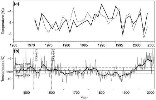The figure is from paper #63.

Climate change mitigation

1. Does replacing coal with wood lower CO2 emissions? Dynamic lifecycle analysis of wood bioenergy

"Because combustion and processing efficiencies for wood are less than coal, the immediate impact of substituting wood for coal is an increase in atmospheric CO2 relative to coal. The payback time for this carbon debt ranges from 44–104 years after clearcut, depending on forest type—assuming the land remains forest. Surprisingly, replanting hardwood forests with fast-growing pine plantations raises the CO2 impact of wood because the equilibrium carbon density of plantations is lower than natural forests. Further, projected growth in wood harvest for bioenergy would increase atmospheric CO2 for at least a century because new carbon debt continuously exceeds NPP. Assuming biofuels are carbon neutral may worsen irreversible impacts of climate change before benefits accrue."

2. Impacts of nationally determined contributions on 2030 global greenhouse gas emissions: uncertainty analysis and distribution of emissions

"We estimate that NDCs project into 56.8–66.5 Gt CO2eq yr−1emissions in 2030 (90% confidence interval), which is higher than previous estimates, and with a larger uncertainty range. Despite these uncertainties, NDCs robustly shift GHG emissions towards emerging and developing countries and reduce international inequalities in per capita GHG emissions. Finally, we stress that current NDCs imply larger emissions reduction rates after 2030 than during the 2010–2030 period if long-term temperature goals are to be fulfilled. Our results highlight four requirements for the forthcoming 'climate regime': a clearer framework regarding future NDCs' design, an increasing participation of emerging and developing countries in the global mitigation effort, an ambitious update mechanism in order to avoid hardly feasible decarbonization rates after 2030 and an anticipation of steep decreases in global emissions after 2030."

3. From appropriate technology to the clean energy economy: renewable energy and environmental politics since the 1970s

4. The reduction in low-frequency noise of horizontal-axis wind turbines by adjusting blade cone angle

5. Federal research, development, and demonstration priorities for carbon dioxide removal in the United States

6. Study on performance enhancement and emission reduction of used fuel-injected motorcycles using bi-fuel gasoline-LPG

7. Response to marine cloud brightening in a multi-model ensemble

8. Social cost of carbon pricing of power sector CO₂: accounting for leakage and other social implications from subnational policies

"Results indicate that CO₂ leakage is possible within and outside the electric sector, ranging from negative 70% to over 80% in our scenarios, with primarily positive leakage outcomes. Typically ignored in policy analysis, leakage would affect CO₂ reduction benefits. We also observe other potential societal effects within and across regions, such as higher electricity prices, changes in power sector investments, and overall consumption losses. Efforts to reduce leakage, such as constraining power imports into the SCC pricing region likely reduce leakage, but could also result in lower net emissions reductions, as well as larger price increases."

9. Economic consequences of global climate change and mitigation on future hydropower generation

10. Impacts of Foreign Direct Investment and Economic Development on Carbon Dioxide Emissions Across Different Population Regimes

11. Promoting firms’ energy-saving behavior: The role of institutional pressures, top management support and financial slack

12. Studying household decision-making context and cooking fuel transition in rural India

13. Assessment of renewable energy expansion potential and its implications on reforming Japan's electricity system

Climate change

14. Climatic and associated cryospheric, biospheric, and hydrological changes on the Tibetan Plateau: a review

15. Climate change projections over China using regional climate models forced by two CMIP5 global models. Part II: projections of future climate

16. Future Caribbean Climates in a World of Rising Temperatures: The 1.5 vs 2.0 Dilemma

Climate Forcings and Feedbacks

17. An assessment of tropospheric water vapor feedback using radiative kernels

"Water vapor feedbacks on different time scales are investigated using radiative kernels applied to the Atmospheric Infrared Sounder (AIRS) and Microwave Limb Sounder (MLS) satellite observations, as well as the Coupled Model Intercomparison Project Phase 5 (CMIP5) model simulation results. We show that the magnitude of short-term global water vapor feedback based on observed interannual variations from 2004 to 2016 is 1.55 ± 0.23 W m^–2 K^–1, while model simulated results derived from the CMIP5 runs driven by observed sea surface temperature range from 0.99 to 1.75 W m^–2 K^–1, with a multi-model-mean of 1.40 W m^–2 K^–1. The long-term water vapor feedbacks derived from the quadrupling of CO₂ runs range from 1.47 to 2.03 W m^–2 K^–1, higher than the short-term counterparts. The systematic difference between short-term and long-term water vapor feedbacks illustrates that care should be taken when inferring long-term feedbacks from interannual variabilities. Also, the magnitudes of the short-term and long-term feedbacks are closely correlated (R = 0.60) across the models, implying that the observed short-term water vapor feedback could be used to constrain the simulated long-term water vapor feedback. Based on satellite observations, the inferred long-term water vapor feedback is about 1.85 ± 0.32 W m^–2 K^–1."

18. Probabilities of causation of climate changes

19. An intraseasonal variability in CO2 over the Arctic induced by the Madden−Julian oscillation

20. Climate Feedback on Aerosol Emission and Atmospheric Concentrations

Temperature and Precipitation

21. Big Jump of Record Warm Global Mean Surface Temperature in 2014-2016 Related to Unusually Large Oceanic Heat Releases

"A 0.24°C jump of record warm global mean surface temperature (GMST) over the past three consecutive record-breaking years (2014-2016) was highly unusual and largely a consequence of an El Niño that released unusually large amounts of ocean heat from the subsurface layer of the northwestern tropical Pacific (NWP). This heat had built up since the 1990s mainly due to greenhouse-gas (GHG) forcing and possible remote oceanic effects. Model simulations and projections suggest that the fundamental cause, and robust predictor of large record-breaking events of GMST in the 21^st century is GHG forcing rather than internal climate variability alone. Such events will increase in frequency, magnitude and duration, as well as impact, in the future unless GHG forcing is reduced."

22. Large-scale pattern of the diurnal temperature range changes over East Asia and Australia in boreal winter: A perspective of atmospheric circulation

23. Temperature–topographic elevation relationship for high mountain terrain: an example from the southeastern Tibetan Plateau

24. Seasonal and elevational contrasts in temperature trends in Central Chile between 1979 and 2015

25. Future changes over the Himalayas: Maximum and minimum temperature

26. Time of emergence in regional precipitation changes: an updated assessment using the CMIP5 multi-model ensemble

27. Future changes in extreme precipitation indices over Korea

28. Regional frequency analysis of extreme rainfall in Sicily (Italy)

29. Decadal change of the south Atlantic ocean Angola–Benguela frontal zone since 1980

30. Do changing weather types explain observed climatic trends in the Rhine basin? An analysis of within and between-type changes

Cryosphere

31. Causes of glacier melt extremes in the Alps since 1949

"Using surface energy balance simulations, we show that three independent drivers control melt: global radiation, latent heat and the amount of snow at the beginning of the melting season. Extremes are governed by large deviations in global radiation combined with sensible heat. Long-term trends are driven by the lengthening of melt duration due to earlier and longer-lasting melting of ice along with melt intensification caused by trends in long-wave irradiance and latent heat due to higher air moisture."

32. Widespread Moulin Formation During Supraglacial Lake Drainages in Greenland

33. Characterizing permafrost active layer dynamics and sensitivity to landscape spatial heterogeneity in Alaska

Hydrosphere

34. Quantifying the sources of uncertainty in an ensemble of hydrological climate-impact projections

35. Groundwater recharge in desert playas: current rates and future effects of climate change

36. Sources of uncertainty in hydrological climate impact assessment: a cross-scale study

Carbon Cycle

37. Simulated impact of glacial runoff on CO₂ uptake in the Gulf of Alaska

38. The Accelerating Land Carbon Sink of the 2000s may not be Driven Predominantly by the Warming Hiatus

"A conceptual model of the annual/seasonal temperature response of respiration suggests that changes in seasonal temperature during this period are unlikely to cause a significant decrease in annual respiration. The ecosystem models suggest that trends in both gross primary production and terrestrial ecosystem respiration slowed down slightly, but the resulting slight acceleration in net ecosystem productivity is insufficient to explain the increasing trend in S_LAND. Instead, the roles of alternative drivers on the accelerating S_LAND seem to be important."

Atmospheric and Oceanic Circulation

39. Contribution of Surface Thermal Forcing to Mixing in the Ocean

40. Towards optimal observational array for dealing with challenges of El Niño-Southern Oscillation predictions due to diversities of El Niño

Extreme Events

41. How does dynamical downscaling affect model biases and future projections of explosive extratropical cyclones along North America’s Atlantic coast?

42. What's the Worst That Could Happen? Re-examining the 24–25 June 1967 Tornado Outbreak Over Western Europe

Climate change impacts

Mankind

43. Hendra Virus Spillover is a Bimodal System Driven by Climatic Factors

44. Modelling maize phenology, biomass growth and yield under contrasting temperature conditions

45. Mapping water availability, cost and projected consumptive use in the eastern United States with comparisons to the west

"Although few administrative limits have been set on water availability in the east, water managers have identified 315 fresh surface water and 398 fresh groundwater basins (with 151 overlapping basins) as areas of concern (AOCs) where water supply challenges exist due to drought related concerns, environmental flows, groundwater overdraft, or salt water intrusion. This highlights a difference in management where AOCs are identified in the east which simply require additional permitting, while in the west strict administrative limits are established. Although the east is generally considered 'water rich' roughly a quarter of the basins were identified as AOCs; however, this is still in strong contrast to the west where 78% of the surface water basins are operating at or near their administrative limit."

Biosphere

46. A positive relationship between spring temperature and productivity in 20 songbird species in the boreal zone

"Anthropogenic climate warming has already affected the population dynamics of numerous species and is predicted to do so also in the future. To predict the effects of climate change, it is important to know whether productivity is linked to temperature, and whether species’ traits affect responses to climate change. To address these objectives, we analysed monitoring data from the Finnish constant effort site ringing scheme collected in 1987–2013 for 20 common songbird species together with climatic data. Warm spring temperature had a positive linear relationship with productivity across the community of 20 species independent of species’ traits (realized thermal niche or migration behaviour), suggesting that even the warmest spring temperatures remained below the thermal optimum for reproduction, possibly due to our boreal study area being closer to the cold edge of all study species’ distributions. The result also suggests a lack of mismatch between the timing of breeding and peak availability of invertebrate food of the study species. Productivity was positively related to annual growth rates in long-distance migrants, but not in short-distance migrants. Across the 27-year study period, temporal trends in productivity were mostly absent. The population sizes of species with colder thermal niches had decreasing trends, which were not related to temperature responses or temporal trends in productivity. The positive connection between spring temperature and productivity suggests that climate warming has potential to increase the productivity in bird species in the boreal zone, at least in the short term."

47. Hillslope topography mediates spatial patterns of ecosystem sensitivity to climate

48. ‘Stick with your own kind, or hang with the locals?’ Implications of shoaling strategy for tropical reef fish on a range-expansion frontline

49. Biological traits explain bryophyte species distributions and responses to forest fragmentation and climatic variation

50. Shock and stabilisation following long-term drought in tropical forest from 15 years of litterfall dynamics

51. Amazon droughts and forest responses: Largely reduced forest photosynthesis but slightly increased canopy greenness during the extreme drought of 2015/2016

52. Anthropogenic nitrogen deposition ameliorates the decline in tree growth caused by a drier climate

53. Trees on the move: using decision theory to compensate for climate change at the regional scale in forest social-ecological systems

54. A unified framework of plant adaptive strategies to drought: crossing scales and disciplines

55. Towards Developing a Mechanistic Understanding of Coral Reef Resilience to Thermal Stress Across Multiple Scales

56. Thermal and hydrologic responses to climate change predict marked alterations in boreal stream invertebrate assemblages

57. The responses of microbial temperature relationships to seasonal change and winter warming in a temperate grassland soil

58. Precipitation frequency alters peatland ecosystem structure and CO2 exchange: contrasting effects on moss, sedge, and shrub communities

59. Highly dynamic wintering strategies in migratory geese: coping with environmental change

"Our findings demonstrate that individual winter strategies are very flexible and able to change over time, suggesting that phenotypic plasticity and cultural transmission are important drivers of strategy choice in this species. Growing benefits from exploratory behaviours, including the ability to track rapid land use changes, may ultimately result in increased resilience to global change."

Other Impacts

60. The sensitivity of US wildfire occurrence to pre-season soil moisture conditions across ecosystems

61. Circumpolar spatio-temporal patterns and contributing climatic factors of wildfire activity in the Arctic tundra from 2001–2015

Other papers

62. Tropical Atlantic climate and ecosystem regime shifts during the Paleocene–Eocene Thermal Maximum

63. Autumn–winter minimum temperature changes in the southern Sikhote-Alin mountain range of northeastern Asia since 1529 AD

64. Memory matters: A case for Granger causality in climate variability studies

from Skeptical Science http://ift.tt/2DCuuF8

A selection of new climate related research articles is shown below.

The figure is from paper #63.

Climate change mitigation

1. Does replacing coal with wood lower CO2 emissions? Dynamic lifecycle analysis of wood bioenergy

"Because combustion and processing efficiencies for wood are less than coal, the immediate impact of substituting wood for coal is an increase in atmospheric CO2 relative to coal. The payback time for this carbon debt ranges from 44–104 years after clearcut, depending on forest type—assuming the land remains forest. Surprisingly, replanting hardwood forests with fast-growing pine plantations raises the CO2 impact of wood because the equilibrium carbon density of plantations is lower than natural forests. Further, projected growth in wood harvest for bioenergy would increase atmospheric CO2 for at least a century because new carbon debt continuously exceeds NPP. Assuming biofuels are carbon neutral may worsen irreversible impacts of climate change before benefits accrue."

2. Impacts of nationally determined contributions on 2030 global greenhouse gas emissions: uncertainty analysis and distribution of emissions

"We estimate that NDCs project into 56.8–66.5 Gt CO2eq yr−1emissions in 2030 (90% confidence interval), which is higher than previous estimates, and with a larger uncertainty range. Despite these uncertainties, NDCs robustly shift GHG emissions towards emerging and developing countries and reduce international inequalities in per capita GHG emissions. Finally, we stress that current NDCs imply larger emissions reduction rates after 2030 than during the 2010–2030 period if long-term temperature goals are to be fulfilled. Our results highlight four requirements for the forthcoming 'climate regime': a clearer framework regarding future NDCs' design, an increasing participation of emerging and developing countries in the global mitigation effort, an ambitious update mechanism in order to avoid hardly feasible decarbonization rates after 2030 and an anticipation of steep decreases in global emissions after 2030."

3. From appropriate technology to the clean energy economy: renewable energy and environmental politics since the 1970s

4. The reduction in low-frequency noise of horizontal-axis wind turbines by adjusting blade cone angle

5. Federal research, development, and demonstration priorities for carbon dioxide removal in the United States

6. Study on performance enhancement and emission reduction of used fuel-injected motorcycles using bi-fuel gasoline-LPG

7. Response to marine cloud brightening in a multi-model ensemble

8. Social cost of carbon pricing of power sector CO₂: accounting for leakage and other social implications from subnational policies

"Results indicate that CO₂ leakage is possible within and outside the electric sector, ranging from negative 70% to over 80% in our scenarios, with primarily positive leakage outcomes. Typically ignored in policy analysis, leakage would affect CO₂ reduction benefits. We also observe other potential societal effects within and across regions, such as higher electricity prices, changes in power sector investments, and overall consumption losses. Efforts to reduce leakage, such as constraining power imports into the SCC pricing region likely reduce leakage, but could also result in lower net emissions reductions, as well as larger price increases."

9. Economic consequences of global climate change and mitigation on future hydropower generation

10. Impacts of Foreign Direct Investment and Economic Development on Carbon Dioxide Emissions Across Different Population Regimes

11. Promoting firms’ energy-saving behavior: The role of institutional pressures, top management support and financial slack

12. Studying household decision-making context and cooking fuel transition in rural India

13. Assessment of renewable energy expansion potential and its implications on reforming Japan's electricity system

Climate change

14. Climatic and associated cryospheric, biospheric, and hydrological changes on the Tibetan Plateau: a review

15. Climate change projections over China using regional climate models forced by two CMIP5 global models. Part II: projections of future climate

16. Future Caribbean Climates in a World of Rising Temperatures: The 1.5 vs 2.0 Dilemma

Climate Forcings and Feedbacks

17. An assessment of tropospheric water vapor feedback using radiative kernels

"Water vapor feedbacks on different time scales are investigated using radiative kernels applied to the Atmospheric Infrared Sounder (AIRS) and Microwave Limb Sounder (MLS) satellite observations, as well as the Coupled Model Intercomparison Project Phase 5 (CMIP5) model simulation results. We show that the magnitude of short-term global water vapor feedback based on observed interannual variations from 2004 to 2016 is 1.55 ± 0.23 W m^–2 K^–1, while model simulated results derived from the CMIP5 runs driven by observed sea surface temperature range from 0.99 to 1.75 W m^–2 K^–1, with a multi-model-mean of 1.40 W m^–2 K^–1. The long-term water vapor feedbacks derived from the quadrupling of CO₂ runs range from 1.47 to 2.03 W m^–2 K^–1, higher than the short-term counterparts. The systematic difference between short-term and long-term water vapor feedbacks illustrates that care should be taken when inferring long-term feedbacks from interannual variabilities. Also, the magnitudes of the short-term and long-term feedbacks are closely correlated (R = 0.60) across the models, implying that the observed short-term water vapor feedback could be used to constrain the simulated long-term water vapor feedback. Based on satellite observations, the inferred long-term water vapor feedback is about 1.85 ± 0.32 W m^–2 K^–1."

18. Probabilities of causation of climate changes

19. An intraseasonal variability in CO2 over the Arctic induced by the Madden−Julian oscillation

20. Climate Feedback on Aerosol Emission and Atmospheric Concentrations

Temperature and Precipitation

21. Big Jump of Record Warm Global Mean Surface Temperature in 2014-2016 Related to Unusually Large Oceanic Heat Releases

"A 0.24°C jump of record warm global mean surface temperature (GMST) over the past three consecutive record-breaking years (2014-2016) was highly unusual and largely a consequence of an El Niño that released unusually large amounts of ocean heat from the subsurface layer of the northwestern tropical Pacific (NWP). This heat had built up since the 1990s mainly due to greenhouse-gas (GHG) forcing and possible remote oceanic effects. Model simulations and projections suggest that the fundamental cause, and robust predictor of large record-breaking events of GMST in the 21^st century is GHG forcing rather than internal climate variability alone. Such events will increase in frequency, magnitude and duration, as well as impact, in the future unless GHG forcing is reduced."

22. Large-scale pattern of the diurnal temperature range changes over East Asia and Australia in boreal winter: A perspective of atmospheric circulation

23. Temperature–topographic elevation relationship for high mountain terrain: an example from the southeastern Tibetan Plateau

24. Seasonal and elevational contrasts in temperature trends in Central Chile between 1979 and 2015

25. Future changes over the Himalayas: Maximum and minimum temperature

26. Time of emergence in regional precipitation changes: an updated assessment using the CMIP5 multi-model ensemble

27. Future changes in extreme precipitation indices over Korea

28. Regional frequency analysis of extreme rainfall in Sicily (Italy)

29. Decadal change of the south Atlantic ocean Angola–Benguela frontal zone since 1980

30. Do changing weather types explain observed climatic trends in the Rhine basin? An analysis of within and between-type changes

Cryosphere

31. Causes of glacier melt extremes in the Alps since 1949

"Using surface energy balance simulations, we show that three independent drivers control melt: global radiation, latent heat and the amount of snow at the beginning of the melting season. Extremes are governed by large deviations in global radiation combined with sensible heat. Long-term trends are driven by the lengthening of melt duration due to earlier and longer-lasting melting of ice along with melt intensification caused by trends in long-wave irradiance and latent heat due to higher air moisture."

32. Widespread Moulin Formation During Supraglacial Lake Drainages in Greenland

33. Characterizing permafrost active layer dynamics and sensitivity to landscape spatial heterogeneity in Alaska

Hydrosphere

34. Quantifying the sources of uncertainty in an ensemble of hydrological climate-impact projections

35. Groundwater recharge in desert playas: current rates and future effects of climate change

36. Sources of uncertainty in hydrological climate impact assessment: a cross-scale study

Carbon Cycle

37. Simulated impact of glacial runoff on CO₂ uptake in the Gulf of Alaska

38. The Accelerating Land Carbon Sink of the 2000s may not be Driven Predominantly by the Warming Hiatus

"A conceptual model of the annual/seasonal temperature response of respiration suggests that changes in seasonal temperature during this period are unlikely to cause a significant decrease in annual respiration. The ecosystem models suggest that trends in both gross primary production and terrestrial ecosystem respiration slowed down slightly, but the resulting slight acceleration in net ecosystem productivity is insufficient to explain the increasing trend in S_LAND. Instead, the roles of alternative drivers on the accelerating S_LAND seem to be important."

Atmospheric and Oceanic Circulation

39. Contribution of Surface Thermal Forcing to Mixing in the Ocean

40. Towards optimal observational array for dealing with challenges of El Niño-Southern Oscillation predictions due to diversities of El Niño

Extreme Events

41. How does dynamical downscaling affect model biases and future projections of explosive extratropical cyclones along North America’s Atlantic coast?

42. What's the Worst That Could Happen? Re-examining the 24–25 June 1967 Tornado Outbreak Over Western Europe

Climate change impacts

Mankind

43. Hendra Virus Spillover is a Bimodal System Driven by Climatic Factors

44. Modelling maize phenology, biomass growth and yield under contrasting temperature conditions

45. Mapping water availability, cost and projected consumptive use in the eastern United States with comparisons to the west

"Although few administrative limits have been set on water availability in the east, water managers have identified 315 fresh surface water and 398 fresh groundwater basins (with 151 overlapping basins) as areas of concern (AOCs) where water supply challenges exist due to drought related concerns, environmental flows, groundwater overdraft, or salt water intrusion. This highlights a difference in management where AOCs are identified in the east which simply require additional permitting, while in the west strict administrative limits are established. Although the east is generally considered 'water rich' roughly a quarter of the basins were identified as AOCs; however, this is still in strong contrast to the west where 78% of the surface water basins are operating at or near their administrative limit."

Biosphere

46. A positive relationship between spring temperature and productivity in 20 songbird species in the boreal zone

"Anthropogenic climate warming has already affected the population dynamics of numerous species and is predicted to do so also in the future. To predict the effects of climate change, it is important to know whether productivity is linked to temperature, and whether species’ traits affect responses to climate change. To address these objectives, we analysed monitoring data from the Finnish constant effort site ringing scheme collected in 1987–2013 for 20 common songbird species together with climatic data. Warm spring temperature had a positive linear relationship with productivity across the community of 20 species independent of species’ traits (realized thermal niche or migration behaviour), suggesting that even the warmest spring temperatures remained below the thermal optimum for reproduction, possibly due to our boreal study area being closer to the cold edge of all study species’ distributions. The result also suggests a lack of mismatch between the timing of breeding and peak availability of invertebrate food of the study species. Productivity was positively related to annual growth rates in long-distance migrants, but not in short-distance migrants. Across the 27-year study period, temporal trends in productivity were mostly absent. The population sizes of species with colder thermal niches had decreasing trends, which were not related to temperature responses or temporal trends in productivity. The positive connection between spring temperature and productivity suggests that climate warming has potential to increase the productivity in bird species in the boreal zone, at least in the short term."

47. Hillslope topography mediates spatial patterns of ecosystem sensitivity to climate

48. ‘Stick with your own kind, or hang with the locals?’ Implications of shoaling strategy for tropical reef fish on a range-expansion frontline

49. Biological traits explain bryophyte species distributions and responses to forest fragmentation and climatic variation

50. Shock and stabilisation following long-term drought in tropical forest from 15 years of litterfall dynamics

51. Amazon droughts and forest responses: Largely reduced forest photosynthesis but slightly increased canopy greenness during the extreme drought of 2015/2016

52. Anthropogenic nitrogen deposition ameliorates the decline in tree growth caused by a drier climate

53. Trees on the move: using decision theory to compensate for climate change at the regional scale in forest social-ecological systems

54. A unified framework of plant adaptive strategies to drought: crossing scales and disciplines

55. Towards Developing a Mechanistic Understanding of Coral Reef Resilience to Thermal Stress Across Multiple Scales

56. Thermal and hydrologic responses to climate change predict marked alterations in boreal stream invertebrate assemblages

57. The responses of microbial temperature relationships to seasonal change and winter warming in a temperate grassland soil

58. Precipitation frequency alters peatland ecosystem structure and CO2 exchange: contrasting effects on moss, sedge, and shrub communities

59. Highly dynamic wintering strategies in migratory geese: coping with environmental change

"Our findings demonstrate that individual winter strategies are very flexible and able to change over time, suggesting that phenotypic plasticity and cultural transmission are important drivers of strategy choice in this species. Growing benefits from exploratory behaviours, including the ability to track rapid land use changes, may ultimately result in increased resilience to global change."

Other Impacts

60. The sensitivity of US wildfire occurrence to pre-season soil moisture conditions across ecosystems

61. Circumpolar spatio-temporal patterns and contributing climatic factors of wildfire activity in the Arctic tundra from 2001–2015

Other papers

62. Tropical Atlantic climate and ecosystem regime shifts during the Paleocene–Eocene Thermal Maximum

63. Autumn–winter minimum temperature changes in the southern Sikhote-Alin mountain range of northeastern Asia since 1529 AD

64. Memory matters: A case for Granger causality in climate variability studies

from Skeptical Science http://ift.tt/2DCuuF8

January 31 lunar eclipse: What scientists can learn

The moon takes on a reddish hue during a lunar eclipse. Image via NASA’s Goddard Space Flight Center.

By Elizabeth Zubritsky, NASA’s Goddard Space Flight Center

The lunar eclipse on January 31, 2018 will give a team of scientists a special opportunity to study the moon using the astronomer’s equivalent of a heat-sensing, or thermal, camera.

Three lunar events will come together in an unusual overlap that’s being playfully called a super blue blood moon. The second full moon in January will take place on the 31st, making it the first blue moon of 2018. It also will be considered a supermoon — one that appears slightly larger and brighter than usual because it occurs when the moon is near its perigee, or the closest point in its orbit to Earth.

In addition, a lunar eclipse will take place in the morning on January 31, temporarily giving the moon a reddish color known as a blood moon.

For the researchers, the eclipse offers a chance to see what happens when the surface of the moon cools quickly. This information will help them understand some of the characteristics of the regolith — the mixture of soil and loose rocks on the surface — and how it changes over time.

Noah Petro is deputy project scientist for NASA’s Lunar Reconnaissance Orbiter, or LRO, at Goddard Space Flight Center in Greenbelt, Maryland. Petro said:

During a lunar eclipse, the temperature swing is so dramatic that it’s as if the surface of the moon goes from being in an oven to being in a freezer in just a few hours.

Stages of the January 31, 2018 “super blue blood moon” (weather permitting) are depicted in Pacific Time with “moonset” times for major cities across the U.S., which affect how much of the event viewers will see. While viewers along the U.S. East Coast will see only the initial stages of the eclipse before moonset, those in the West and Hawaii will see most or all of the lunar eclipse phases before dawn. Image via NASA.

Normally, the transitions into and out of darkness, and the temperature changes that go with them, are spread out over the course of a lunar day, which lasts 29-and-a-half Earth days. A lunar eclipse shifts these changes into high gear.

From the Haleakala Observatory on the island of Maui in Hawaii, the team will conduct their investigations at invisible wavelengths where heat is sensed. They’ve done this kind of study a few times already, singling out individual lunar locations to see how well they retain warmth throughout the eclipse.

Paul Hayne, of the Laboratory for Atmospheric and Space Physics at the University of Colorado Boulder, said:

The whole character of the moon changes when we observe with a thermal camera during an eclipse. In the dark, many familiar craters and other features can’t be seen, and the normally non-descript areas around some craters start to ‘glow,’ because the rocks there are still warm.

How quickly or slowly the surface loses heat depends on the sizes of the rocks and the characteristics of the material, including its composition, how porous it is and how fluffy it is.

Lunar scientists already know a lot about the day-to-night and seasonal temperature changes from the data collected by LRO’s Diviner instrument since 2009. Those longer-term variations reveal information about larger features and the bulk properties of the top few inches of regolith. The short-term changes due to the eclipse will get at details of the fine material and the very top layer of the regolith.

By comparing the two types of observations, the team is able to look at variations in particular areas — say, the lunar swirls at Reiner Gamma or an impact crater and the loose debris around it.

This kind of information is useful for practical purposes such as scouting out suitable landing sites. It also helps researchers understand the evolution of the surface of the moon. Petro said:

These studies will help us tell the story of how impacts large and small are changing the surface of the Moon over geological time.

Bottom line: Scientists will use a thermal camera to study the moon during the lunar eclipse of January 31, 2018.

from EarthSky http://ift.tt/2E6XxgM

The moon takes on a reddish hue during a lunar eclipse. Image via NASA’s Goddard Space Flight Center.

By Elizabeth Zubritsky, NASA’s Goddard Space Flight Center

The lunar eclipse on January 31, 2018 will give a team of scientists a special opportunity to study the moon using the astronomer’s equivalent of a heat-sensing, or thermal, camera.

Three lunar events will come together in an unusual overlap that’s being playfully called a super blue blood moon. The second full moon in January will take place on the 31st, making it the first blue moon of 2018. It also will be considered a supermoon — one that appears slightly larger and brighter than usual because it occurs when the moon is near its perigee, or the closest point in its orbit to Earth.

In addition, a lunar eclipse will take place in the morning on January 31, temporarily giving the moon a reddish color known as a blood moon.

For the researchers, the eclipse offers a chance to see what happens when the surface of the moon cools quickly. This information will help them understand some of the characteristics of the regolith — the mixture of soil and loose rocks on the surface — and how it changes over time.

Noah Petro is deputy project scientist for NASA’s Lunar Reconnaissance Orbiter, or LRO, at Goddard Space Flight Center in Greenbelt, Maryland. Petro said:

During a lunar eclipse, the temperature swing is so dramatic that it’s as if the surface of the moon goes from being in an oven to being in a freezer in just a few hours.

Stages of the January 31, 2018 “super blue blood moon” (weather permitting) are depicted in Pacific Time with “moonset” times for major cities across the U.S., which affect how much of the event viewers will see. While viewers along the U.S. East Coast will see only the initial stages of the eclipse before moonset, those in the West and Hawaii will see most or all of the lunar eclipse phases before dawn. Image via NASA.

Normally, the transitions into and out of darkness, and the temperature changes that go with them, are spread out over the course of a lunar day, which lasts 29-and-a-half Earth days. A lunar eclipse shifts these changes into high gear.

From the Haleakala Observatory on the island of Maui in Hawaii, the team will conduct their investigations at invisible wavelengths where heat is sensed. They’ve done this kind of study a few times already, singling out individual lunar locations to see how well they retain warmth throughout the eclipse.

Paul Hayne, of the Laboratory for Atmospheric and Space Physics at the University of Colorado Boulder, said:

The whole character of the moon changes when we observe with a thermal camera during an eclipse. In the dark, many familiar craters and other features can’t be seen, and the normally non-descript areas around some craters start to ‘glow,’ because the rocks there are still warm.

How quickly or slowly the surface loses heat depends on the sizes of the rocks and the characteristics of the material, including its composition, how porous it is and how fluffy it is.

Lunar scientists already know a lot about the day-to-night and seasonal temperature changes from the data collected by LRO’s Diviner instrument since 2009. Those longer-term variations reveal information about larger features and the bulk properties of the top few inches of regolith. The short-term changes due to the eclipse will get at details of the fine material and the very top layer of the regolith.

By comparing the two types of observations, the team is able to look at variations in particular areas — say, the lunar swirls at Reiner Gamma or an impact crater and the loose debris around it.

This kind of information is useful for practical purposes such as scouting out suitable landing sites. It also helps researchers understand the evolution of the surface of the moon. Petro said:

These studies will help us tell the story of how impacts large and small are changing the surface of the Moon over geological time.

Bottom line: Scientists will use a thermal camera to study the moon during the lunar eclipse of January 31, 2018.

from EarthSky http://ift.tt/2E6XxgM