Where does Mars’ methane come from? Not wind

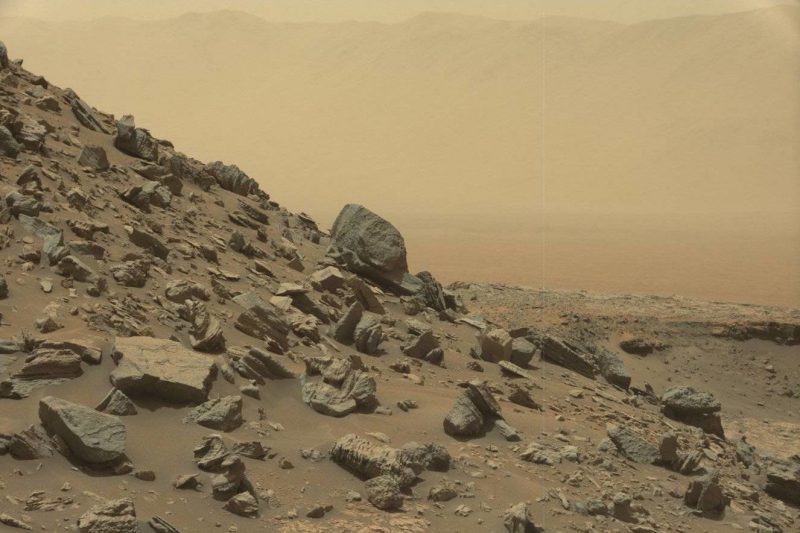
Mars is a rocky world, and some scientists have theorized that erosion by wind causes Mars rocks to produce methane. But a new study from Newcastle University refutes that. Image via NASA/JPL-Caltech/Phys.org.

What is producing methane on Mars? That is a question that scientists have been trying to answer for quite some time now. There are various possibilities, both geological and biological, but narrowing them down has been a challenge. Could it really be a sign of … life? Now, a new study has shown that at least one of the geological scenarios is very unlikely: wind erosion of rocks.

Researchers at Newcastle University in the U.K. published their peer-reviewed findings in Scientific Reports on June 3, 2019, and a new press release was issued on August 12, 2019. From the article abstract:

Seasonal changes in methane background levels and methane spikes have been detected in situ a metre above the martian surface, and larger methane plumes detected via ground-based remote sensing, however their origin have not yet been adequately explained. Proposed methane sources include the UV irradiation of meteoritic-derived organic matter, hydrothermal reactions with olivine, organic breakdown via meteoroid impact, release from gas hydrates, biological production, or the release of methane from fluid inclusions in basalt during aeolian erosion. Here we quantify for the first time the potential importance of aeolian abrasion as a mechanism for releasing trapped methane from within rocks, by coupling estimates of present day surface wind abrasion with the methane contents of a variety of martian meteorites, analogue terrestrial basalts and analogue terrestrial sedimentary rocks. We demonstrate that the abrasion of basalt under present day Martian rates of aeolian erosion is highly unlikely to produce detectable changes in methane concentrations in the atmosphere. We further show that, although there is a greater potential for methane production from the aeolian abrasion of certain sedimentary rocks, to produce the magnitude of methane concentrations analysed by the Curiosity rover they would have to contain methane in similar concentrations as economic reserved of biogenic/thermogenic deposits on Earth. Therefore we suggest that aeolian abrasion is an unlikely origin of the methane detected in the martian atmosphere, and that other methane sources are required.

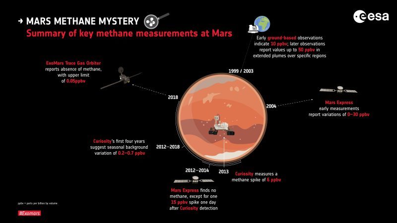
A history of key methane measurements on Mars from 1999 to 2018. Image via ESA.

One of the more recent theories was that wind erosion of rocks could produce the methane detected in the lower atmosphere. But the team’s findings showed that it wouldn’t be able to produce methane in the amounts observed, according to Jon Telling, a geochemist at Newcastle University:

The questions are – where is this methane coming from, and is the source biological? That’s a massive question and to get to the answer we need to rule out lots of other factors first.

We realized one potential source of the methane that people hadn’t really looked at in any detail before was wind erosion, releasing gases trapped within rocks. High resolution imagery from orbit over the last decade have shown that winds on Mars can drive much higher local rates of sand movement, and hence potential rates of sand erosion, than previously recognised.

In fact, in a few cases, the rate of erosion is estimated to be comparable to those of cold and arid sand dune fields on Earth.

Using the data available, we estimated rates of erosion on the surface of Mars and how important it could be in releasing methane.

And taking all that into account we found it was very unlikely to be the source.

What’s important about this is that it strengthens the argument that the methane must be coming from a different source. Whether or not that’s biological, we still don’t know.

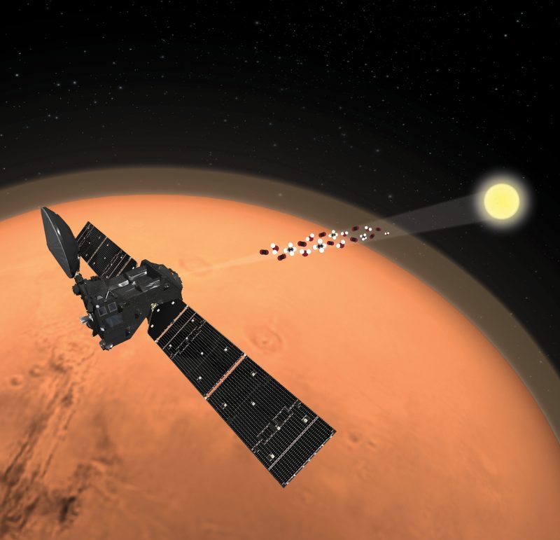
Artist’s concept of ESA’s Trace Gas Orbiter, part of the ExoMars mission, analyzing the Martian atmosphere. Image via ESA/ATG MediaLab.

Observations from both orbiting spacecraft and the Curiosity rover, as well as telescopes on Earth, have shown that methane levels in the Martian atmosphere appear to be seasonal, peaking in the summer and fading again in the winter. Just why that is isn’t known yet, but it indicates a regular process is occurring, whether geological or biological. Oddly, ESA’s Trace Gas Orbiter (TGO) hasn’t detected any methane yet, although that is one of its main objectives. But that may simply be because of the seasonality of the methane, or because TGO focuses its observations on the upper levels of the atmosphere, and most of the other methane detections have been closer to the ground.

Most scientists now think the methane originates from underground, perhaps as ice clathrates that thaw in the summer and release methane, or maybe a biological source that responds to the warmer temperatures. Even if the methane is bound up in clathrates, the actual origin of it could still be either geological of biological (ancient life). Or it may be produced by warm groundwater interacting with olivine in rocks. If so, that would indicate that there is still some residual geological activity below Mars’ surface, and that itself could provide a habitable environment for microorganisms, even if they didn’t actually produce the methane. Other causes, such as meteorites or comets, probably wouldn’t produce enough of the gas to match observations, either, according to recent studies.

Last April, a new report showed that a spike in methane levels was detected at the same time – for the first time – by both the Curiosity rover and the orbiting Mars Express back in 2013. And last June, Curiosity detected its largest-ever measurement of methane so far. Why are there these peaks in methane emissions, only for the gas to virtually disappear afterwards? There is still a lot we don’t know, as Emmal Safi, a postdoctoral researcher at Newcastle University, indicated:

It’s still an open question. Our paper is just a little part of a much bigger story.

Ultimately, what we’re trying to discover is if there’s the possibility of life existing on planets other than our own, either living now or maybe life in the past that is now preserved as fossils or chemical signatures.

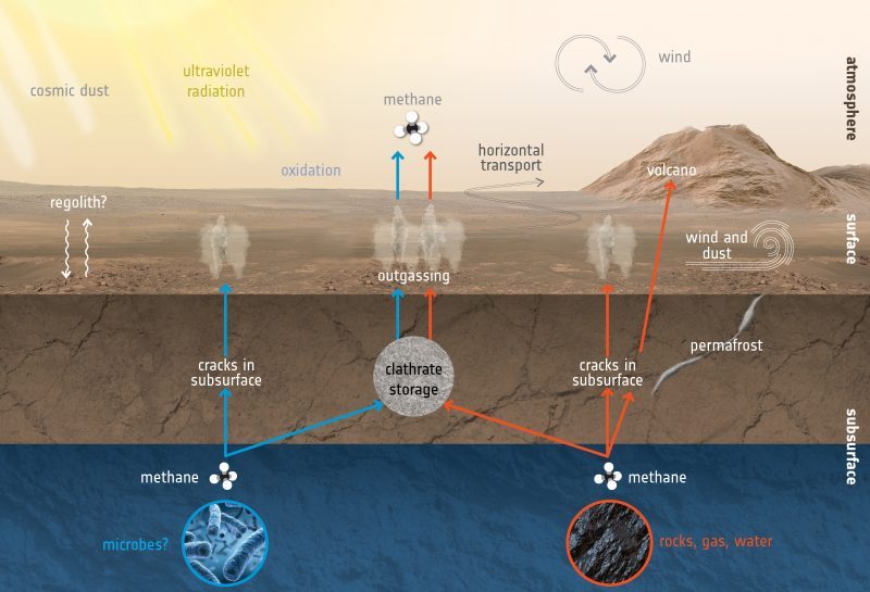
Illustration depicting what processes could create and destroy methane on Mars. The methane most likely originates from below the surface and is released into the atmosphere through subsurface cracks. Image via ESA.

The idea that Mars’ methane might come from life is an exciting one, of course, since most of the methane on Earth is produced by living organisms. But non-biological explanations would need to be eliminated first. The research from Newcastle University shows that at least one of the possible geological explanations for the methane is unlikely, but there is still a lot of work for scientists to do to determine just what is producing it.

Bottom line: This new study would seem to eliminate one possible source of Mars’ methane: wind erosion of rocks on the surface. This bolsters the probability that the methane originates from underground.

Source: Aeolian abrasion of rocks as a mechanism to produce methane in the Martian atmosphere

Via Newcastle University

from EarthSky https://ift.tt/2MsFzMI

Mars is a rocky world, and some scientists have theorized that erosion by wind causes Mars rocks to produce methane. But a new study from Newcastle University refutes that. Image via NASA/JPL-Caltech/Phys.org.

What is producing methane on Mars? That is a question that scientists have been trying to answer for quite some time now. There are various possibilities, both geological and biological, but narrowing them down has been a challenge. Could it really be a sign of … life? Now, a new study has shown that at least one of the geological scenarios is very unlikely: wind erosion of rocks.

Researchers at Newcastle University in the U.K. published their peer-reviewed findings in Scientific Reports on June 3, 2019, and a new press release was issued on August 12, 2019. From the article abstract:

Seasonal changes in methane background levels and methane spikes have been detected in situ a metre above the martian surface, and larger methane plumes detected via ground-based remote sensing, however their origin have not yet been adequately explained. Proposed methane sources include the UV irradiation of meteoritic-derived organic matter, hydrothermal reactions with olivine, organic breakdown via meteoroid impact, release from gas hydrates, biological production, or the release of methane from fluid inclusions in basalt during aeolian erosion. Here we quantify for the first time the potential importance of aeolian abrasion as a mechanism for releasing trapped methane from within rocks, by coupling estimates of present day surface wind abrasion with the methane contents of a variety of martian meteorites, analogue terrestrial basalts and analogue terrestrial sedimentary rocks. We demonstrate that the abrasion of basalt under present day Martian rates of aeolian erosion is highly unlikely to produce detectable changes in methane concentrations in the atmosphere. We further show that, although there is a greater potential for methane production from the aeolian abrasion of certain sedimentary rocks, to produce the magnitude of methane concentrations analysed by the Curiosity rover they would have to contain methane in similar concentrations as economic reserved of biogenic/thermogenic deposits on Earth. Therefore we suggest that aeolian abrasion is an unlikely origin of the methane detected in the martian atmosphere, and that other methane sources are required.

A history of key methane measurements on Mars from 1999 to 2018. Image via ESA.

One of the more recent theories was that wind erosion of rocks could produce the methane detected in the lower atmosphere. But the team’s findings showed that it wouldn’t be able to produce methane in the amounts observed, according to Jon Telling, a geochemist at Newcastle University:

The questions are – where is this methane coming from, and is the source biological? That’s a massive question and to get to the answer we need to rule out lots of other factors first.

We realized one potential source of the methane that people hadn’t really looked at in any detail before was wind erosion, releasing gases trapped within rocks. High resolution imagery from orbit over the last decade have shown that winds on Mars can drive much higher local rates of sand movement, and hence potential rates of sand erosion, than previously recognised.

In fact, in a few cases, the rate of erosion is estimated to be comparable to those of cold and arid sand dune fields on Earth.

Using the data available, we estimated rates of erosion on the surface of Mars and how important it could be in releasing methane.

And taking all that into account we found it was very unlikely to be the source.

What’s important about this is that it strengthens the argument that the methane must be coming from a different source. Whether or not that’s biological, we still don’t know.

Artist’s concept of ESA’s Trace Gas Orbiter, part of the ExoMars mission, analyzing the Martian atmosphere. Image via ESA/ATG MediaLab.

Observations from both orbiting spacecraft and the Curiosity rover, as well as telescopes on Earth, have shown that methane levels in the Martian atmosphere appear to be seasonal, peaking in the summer and fading again in the winter. Just why that is isn’t known yet, but it indicates a regular process is occurring, whether geological or biological. Oddly, ESA’s Trace Gas Orbiter (TGO) hasn’t detected any methane yet, although that is one of its main objectives. But that may simply be because of the seasonality of the methane, or because TGO focuses its observations on the upper levels of the atmosphere, and most of the other methane detections have been closer to the ground.

Most scientists now think the methane originates from underground, perhaps as ice clathrates that thaw in the summer and release methane, or maybe a biological source that responds to the warmer temperatures. Even if the methane is bound up in clathrates, the actual origin of it could still be either geological of biological (ancient life). Or it may be produced by warm groundwater interacting with olivine in rocks. If so, that would indicate that there is still some residual geological activity below Mars’ surface, and that itself could provide a habitable environment for microorganisms, even if they didn’t actually produce the methane. Other causes, such as meteorites or comets, probably wouldn’t produce enough of the gas to match observations, either, according to recent studies.

Last April, a new report showed that a spike in methane levels was detected at the same time – for the first time – by both the Curiosity rover and the orbiting Mars Express back in 2013. And last June, Curiosity detected its largest-ever measurement of methane so far. Why are there these peaks in methane emissions, only for the gas to virtually disappear afterwards? There is still a lot we don’t know, as Emmal Safi, a postdoctoral researcher at Newcastle University, indicated:

It’s still an open question. Our paper is just a little part of a much bigger story.

Ultimately, what we’re trying to discover is if there’s the possibility of life existing on planets other than our own, either living now or maybe life in the past that is now preserved as fossils or chemical signatures.

Illustration depicting what processes could create and destroy methane on Mars. The methane most likely originates from below the surface and is released into the atmosphere through subsurface cracks. Image via ESA.

The idea that Mars’ methane might come from life is an exciting one, of course, since most of the methane on Earth is produced by living organisms. But non-biological explanations would need to be eliminated first. The research from Newcastle University shows that at least one of the possible geological explanations for the methane is unlikely, but there is still a lot of work for scientists to do to determine just what is producing it.

Bottom line: This new study would seem to eliminate one possible source of Mars’ methane: wind erosion of rocks on the surface. This bolsters the probability that the methane originates from underground.

Source: Aeolian abrasion of rocks as a mechanism to produce methane in the Martian atmosphere

Via Newcastle University

from EarthSky https://ift.tt/2MsFzMI

Moon sweeps past planet Uranus

Our chart – above – shows the moon in the early morning sky on August 21, 22 and 23. The green line represents the ecliptic, or approximate path of the sun, moon and planets across our sky. On the mornings of August 21 and 22, you’ll find the waxing gibbous moon sweeping close to the planet Uranus. They’ll be up late at night, too, but low in the sky. You’ll have a better view of them in the wee hours, or before dawn breaks.

Of course, the moon and urnaus are nowhere near each other in space. The moon, our closest celestial neighbor, lies a little less than 250,000 miles (400,000 km) from Earth. Uranus, the seventh planet outward from the sun, lodges well over 7,000 times the moon’s distance from us.

Also, don’t expect to view Uranus with the unaided eye. People with exceptional eyesight might be able to see Uranus as a faint speck of light on a dark, moonless night. Most likely, you would need binoculars (at least) and a steady hand (or a tripod) to see Uranus with the nearby bright moon obscuring this world these next several mornings. For that matter, you’ll probably need binoculars to spot Uranus on most any night. For the ultimate challenge challenge – catching Uranus with the eye alone – try your luck when the moon leaves this part of the sky, say, around new moon at the end of August. Read more: 2019’s closest new moon on August 30

Although Uranus looks like a faint star, even through binoculars, that’s only because this distant world resides in the outskirts of our solar system, at about 19 astronomical units (AU) from the sun. Uranus’ diameter is actually 4 times greater than Earth’s diameter, and its surface area some 16 times greater than that of Earth.

Most of us need binoculars and a sky chart to see this faint world that lurks at the threshold of visibility in our sky. Even through binoculars, though, Uranus appears no brighter than a dim star. You’ll need a telescope magnifying at least 100 times and a steady sky free of atmospheric disturbance to resolve Uranus into a tiny disk.

Uranus will reside in front of the constellation Aries the Ram for years to come, so a good familiarity with this constellation is your ticket to locating this faint world. For a detailed sky chart of Aries, click on The Sky Live; and for a sky chart showing Uranus’ position from 2019 to 2032, click on Naked Eye Planets.

A dark, moonless night provides your best chance of catching Uranus, which is hard to see with the unaided eye but easy to spot with binoculars. Uranus is lightly south of the ecliptic, as we point out on the sky chart. Uranus forms a triangle with two stars that are almost the same brightness as Uranus: 19 Arietis (abbreviated 19 Ari) and HD 12489. Chart via the IAU.

Despite the moonlight, you might be able to make out the Pleiades star cluster (in the constellation Taurus), and the constellation Aries’ brightest star, Hamal (Alpha Arietis), to the west of the Pleiades cluster. In fact, you might even be able to see the three stars outlining the Ram’s Head: Hamal (Alpha Arietis), Sheratan (Beta Arietis), and Mesartim (Gamma Arietis).

If you can identify those Aries’ stars, you are well on your way to star-hopping to Uranus. Your next move is to find the dim star Iota Arietis (abbreviated Iota on the above sky chart), which is only a touch south of the star Mesartim (sometimes spelled Mesarthim). Iota Arietis, though faint, is clearly visible in a dark, moonless sky. An imaginary line drawn from Mesartim through Iota Arietis points in the vicinity of the planet Uranus, and the two faint stars making a triangle with Uranus: 19 Arietis and HD 12489.

These two stars forming a triangle with Uranus pretty much match Uranus in magnitude. They all hover around 6th-magnitude in brightness, near the limit of naked-eye visibility. By good fortune, this triangle fits rather readily within a single binocular field, simplifying our search for Uranus, the ice giant planet.

Click here to know the moon’s present distance from Earth in miles, km, or in astronomical units.

Click here to know the the planet Uranus’ present distance from Earth in astronomical units.

Bottom line: Before dawn on August 21 and 22, 2019, let the moon guide you to the constellation Aries the Ram. When the moon moves away, try star-hopping to the planet Uranus using guide stars within the constellation Aries the Ram. Good luck!

from EarthSky https://ift.tt/2HdRmu4

Our chart – above – shows the moon in the early morning sky on August 21, 22 and 23. The green line represents the ecliptic, or approximate path of the sun, moon and planets across our sky. On the mornings of August 21 and 22, you’ll find the waxing gibbous moon sweeping close to the planet Uranus. They’ll be up late at night, too, but low in the sky. You’ll have a better view of them in the wee hours, or before dawn breaks.

Of course, the moon and urnaus are nowhere near each other in space. The moon, our closest celestial neighbor, lies a little less than 250,000 miles (400,000 km) from Earth. Uranus, the seventh planet outward from the sun, lodges well over 7,000 times the moon’s distance from us.

Also, don’t expect to view Uranus with the unaided eye. People with exceptional eyesight might be able to see Uranus as a faint speck of light on a dark, moonless night. Most likely, you would need binoculars (at least) and a steady hand (or a tripod) to see Uranus with the nearby bright moon obscuring this world these next several mornings. For that matter, you’ll probably need binoculars to spot Uranus on most any night. For the ultimate challenge challenge – catching Uranus with the eye alone – try your luck when the moon leaves this part of the sky, say, around new moon at the end of August. Read more: 2019’s closest new moon on August 30

Although Uranus looks like a faint star, even through binoculars, that’s only because this distant world resides in the outskirts of our solar system, at about 19 astronomical units (AU) from the sun. Uranus’ diameter is actually 4 times greater than Earth’s diameter, and its surface area some 16 times greater than that of Earth.

Most of us need binoculars and a sky chart to see this faint world that lurks at the threshold of visibility in our sky. Even through binoculars, though, Uranus appears no brighter than a dim star. You’ll need a telescope magnifying at least 100 times and a steady sky free of atmospheric disturbance to resolve Uranus into a tiny disk.

Uranus will reside in front of the constellation Aries the Ram for years to come, so a good familiarity with this constellation is your ticket to locating this faint world. For a detailed sky chart of Aries, click on The Sky Live; and for a sky chart showing Uranus’ position from 2019 to 2032, click on Naked Eye Planets.

A dark, moonless night provides your best chance of catching Uranus, which is hard to see with the unaided eye but easy to spot with binoculars. Uranus is lightly south of the ecliptic, as we point out on the sky chart. Uranus forms a triangle with two stars that are almost the same brightness as Uranus: 19 Arietis (abbreviated 19 Ari) and HD 12489. Chart via the IAU.

Despite the moonlight, you might be able to make out the Pleiades star cluster (in the constellation Taurus), and the constellation Aries’ brightest star, Hamal (Alpha Arietis), to the west of the Pleiades cluster. In fact, you might even be able to see the three stars outlining the Ram’s Head: Hamal (Alpha Arietis), Sheratan (Beta Arietis), and Mesartim (Gamma Arietis).

If you can identify those Aries’ stars, you are well on your way to star-hopping to Uranus. Your next move is to find the dim star Iota Arietis (abbreviated Iota on the above sky chart), which is only a touch south of the star Mesartim (sometimes spelled Mesarthim). Iota Arietis, though faint, is clearly visible in a dark, moonless sky. An imaginary line drawn from Mesartim through Iota Arietis points in the vicinity of the planet Uranus, and the two faint stars making a triangle with Uranus: 19 Arietis and HD 12489.

These two stars forming a triangle with Uranus pretty much match Uranus in magnitude. They all hover around 6th-magnitude in brightness, near the limit of naked-eye visibility. By good fortune, this triangle fits rather readily within a single binocular field, simplifying our search for Uranus, the ice giant planet.

Click here to know the moon’s present distance from Earth in miles, km, or in astronomical units.

Click here to know the the planet Uranus’ present distance from Earth in astronomical units.

Bottom line: Before dawn on August 21 and 22, 2019, let the moon guide you to the constellation Aries the Ram. When the moon moves away, try star-hopping to the planet Uranus using guide stars within the constellation Aries the Ram. Good luck!

from EarthSky https://ift.tt/2HdRmu4

Scientists detect a black hole swallowing a neutron star

Artist’s concept of a scene that could occur when a black hole and neutron star meet, in a galaxy far, far away. Image via ANU.

Scientists announced today (August 19, 2019) that they believe they’ve detected a black hole swallowing a neutron star. Both of these objects represent the super-dense remains of dead stars. In this case, they reside 900 million light-years away – far from our Milky Way galaxy – so we know their meeting, if it happened, took place 900 million years ago. It has taken all those years for gravitational waves – ripples in space and time created in their meeting – to travel to Earth, to be sensed finally on Wednesday, August 14, 2019, via a trio of gravitational-wave detectors in the United States and Italy.

Scientists are sounding cautiously excited about this detection. Writing in Science on August 16, 2019, Andrew Cho said:

Gravitational-wave hunters may have spotted their most exotic quarry yet. On 14 August at 5:10:39 p.m. EDT, a trio of gigantic detectors in the United States and Italy detected a pulse of gravitational waves – ripples in space itself – apparently set off when a black hole and a neutron star spiraled into each other about 900 million light-years away. Observers had previously spotted numerous mergers of black holes and one merger of neutron stars, but never a combination. The new find could give new insights into neutron stars, which are made of the densest matter in the cosmos.

The August 14 gravitational wave detections were made by the Advanced Laser Interferometer Gravitational-wave Observatory (LIGO), composed of twin gravitational wave detectors in the U.S., as well as by the European Gravitational Observatory’s Virgo detector in Italy.

There’s every reason to think black holes do swallow neutron stars sometimes, just as they might swallow anything else that comes too close to them. The gravitational waves indicate that something happened, and analysis suggests masses for the merging objects in line with those of black holes and neutron stars. Susan Scott, who is the leader of the General Relativity Theory and Data Analysis Group at the Australian National University, has been involved in the analysis. In a statement released August 19, 2019, Scott said:

About 900 million years ago, this black hole ate a very dense star, known as a neutron star, like Pac-man – possibly snuffing out the star instantly.

So both LIGO and Virgo picked up signals on August 14 from a black hole/neutron star merger (if that’s what it was). Scott sounded confident when she commented that this most recent detection completes a trifecta of observations on these scientists’ original wish list: black holes with black holes, neutron stars with neutron stars, and now a black hole with a neutron star. She added that there’s been no visual confirmation of the black hole/neutron star merger, despite the fact that:

The ANU SkyMapper Telescope [an automated wide-field survey telescope ] responded to the detection alert and scanned the entire likely region of space where the event occurred…

And she said scientists are still analyzing the data to confirm the exact size of the two objects, but initial findings indicate the very strong likelihood of a black hole enveloping a neutron star. The final results are expected to be published in scientific journals. Scott explained:

Scientists have never detected a black hole smaller than five solar masses or a neutron star larger than about 2.5 times the mass of our sun.

Based on this experience, we’re very confident that we’ve just detected a black hole gobbling up a neutron star.

However, there is the slight but intriguing possibility that the swallowed object was a very light black hole – much lighter than any other black hole we know about in the universe. That would be a truly awesome consolation prize.

What do we know of black hole/neutron star mergers? One way to study them from Earth is to create simulations, like this one via Simulating Extreme Spacetimes (CC BY-NC 3)/Science.

Bottom line: For the first time, scientists have detected gravitational waves from a black hole/neutron star collision.

Via ANU

from EarthSky https://ift.tt/2ZhVK1H

Artist’s concept of a scene that could occur when a black hole and neutron star meet, in a galaxy far, far away. Image via ANU.

Scientists announced today (August 19, 2019) that they believe they’ve detected a black hole swallowing a neutron star. Both of these objects represent the super-dense remains of dead stars. In this case, they reside 900 million light-years away – far from our Milky Way galaxy – so we know their meeting, if it happened, took place 900 million years ago. It has taken all those years for gravitational waves – ripples in space and time created in their meeting – to travel to Earth, to be sensed finally on Wednesday, August 14, 2019, via a trio of gravitational-wave detectors in the United States and Italy.

Scientists are sounding cautiously excited about this detection. Writing in Science on August 16, 2019, Andrew Cho said:

Gravitational-wave hunters may have spotted their most exotic quarry yet. On 14 August at 5:10:39 p.m. EDT, a trio of gigantic detectors in the United States and Italy detected a pulse of gravitational waves – ripples in space itself – apparently set off when a black hole and a neutron star spiraled into each other about 900 million light-years away. Observers had previously spotted numerous mergers of black holes and one merger of neutron stars, but never a combination. The new find could give new insights into neutron stars, which are made of the densest matter in the cosmos.

The August 14 gravitational wave detections were made by the Advanced Laser Interferometer Gravitational-wave Observatory (LIGO), composed of twin gravitational wave detectors in the U.S., as well as by the European Gravitational Observatory’s Virgo detector in Italy.

There’s every reason to think black holes do swallow neutron stars sometimes, just as they might swallow anything else that comes too close to them. The gravitational waves indicate that something happened, and analysis suggests masses for the merging objects in line with those of black holes and neutron stars. Susan Scott, who is the leader of the General Relativity Theory and Data Analysis Group at the Australian National University, has been involved in the analysis. In a statement released August 19, 2019, Scott said:

About 900 million years ago, this black hole ate a very dense star, known as a neutron star, like Pac-man – possibly snuffing out the star instantly.

So both LIGO and Virgo picked up signals on August 14 from a black hole/neutron star merger (if that’s what it was). Scott sounded confident when she commented that this most recent detection completes a trifecta of observations on these scientists’ original wish list: black holes with black holes, neutron stars with neutron stars, and now a black hole with a neutron star. She added that there’s been no visual confirmation of the black hole/neutron star merger, despite the fact that:

The ANU SkyMapper Telescope [an automated wide-field survey telescope ] responded to the detection alert and scanned the entire likely region of space where the event occurred…

And she said scientists are still analyzing the data to confirm the exact size of the two objects, but initial findings indicate the very strong likelihood of a black hole enveloping a neutron star. The final results are expected to be published in scientific journals. Scott explained:

Scientists have never detected a black hole smaller than five solar masses or a neutron star larger than about 2.5 times the mass of our sun.

Based on this experience, we’re very confident that we’ve just detected a black hole gobbling up a neutron star.

However, there is the slight but intriguing possibility that the swallowed object was a very light black hole – much lighter than any other black hole we know about in the universe. That would be a truly awesome consolation prize.

What do we know of black hole/neutron star mergers? One way to study them from Earth is to create simulations, like this one via Simulating Extreme Spacetimes (CC BY-NC 3)/Science.

Bottom line: For the first time, scientists have detected gravitational waves from a black hole/neutron star collision.

Via ANU

from EarthSky https://ift.tt/2ZhVK1H

Market Forces and Coal

Following defeat of the Australian Labor Party in the Federal election a leading Member has suggested that the Party should not rely on the use of Market Forces as the basis for curbing emissions.  This would be a mistake since it is these forces, particularly those of supply and demand, which governments can not resist - no matter how ill-disposed to rapid reduction of greenhouse gas emissions they may be.

Supply and demand are influenced by price, reliability, cost to use, appearance and many other comparative factors.  Simply put, a manufacturer will not produce goods or services unless cost of production enables him to compete profitably with other producers. Consumers are unlikely to purchase a product unless it is deemed to have advantages over other products. 

Into this mix has been inserted new, highly disruptive, though still evolving technology in the form of renewable energy generation.  It is disruptive because it enables radical departure from existing, often long-standing technology to which we have all become accustomed.  It offers cheaper, more efficient production of goods and services which can be supplied to consumers at lower prices, though more profitably.  Nowhere is this more evident than in the generation, storage and use of electricity.

Coal

Demand for coal is primarily created by demand for electricity, steel, bitumen and other products.  The fact that the Adani coal mine will be built and will export coal to India is a natural response to this demand – and the demand for more jobs in Regional Queensland.  It will not help reduce greenhouse gas emissions but it is a natural response to market forces.

Demand for the end-products of coal is likely to increase in coming years because of a growing population and expanding economic growth, giving the impression that the future of the coal industry is secure.  Not so, because electricity generated from renewable sources, primarily wind and solar, is now cheaper than electricity generated from new coal-fired power stations while old power stations are closing because essential maintenance is becoming more pervasive and expensive.

Australia is unquestionably the worlds’ leading exporter of coal.  In 2017 it exported 202 million tonnes of thermal coal which was used to generate electricity and 177 million tonnes of coking coal used for smelting and other purposes.  In addition, Australian coal mines produced and sold some 44 million tonnes for domestic consumption, mostly for power generation.  However coal production is prone to contraction due to falling internal and external demand and other factors such as price or availability of substitutes such as Liquified Natural Gas.

Domestic Demand

In 2018 Australia had 19 coal fired power stations in operation, generating about 62% of its electricity with the balance coming from oil and gas-fired power stations (23%) and renewables (15%).  

Fig 1.  Rapid expansion of large-scale solar Photovoltaic (PV) generation is expected by the end of 2019 with new capacity of 1,570 MW commissioned in 2018 and 4 - 5,000 MW likely to complete in 2019.  Source of graphic:  Wikipedia.

Australia's coal-fired power stations have a nominal capacity to generate 24,970 MW.  With closure of 4 stations likely by 2030 (5,654 MW) and a further 11 (16,151 MW) closing by 2040, leaving 4 stations (3,165 MW) which may operate beyond 2040.  It is possible, indeed likely, that all 19 power stations could close by 2030 without causing any failure to meet national demand for electricity. The reason for this is, as shown in Fig 2. below, the investment pipeline in renewable energy has a generating capacity of 29,307 MW, exceeding the nominal capacity of coal fired power stations now in operation.

Fig. 2.  The Pipeline comprises approved projects which have commenced/not commenced but are likely to be commissioned by 2025.  It excludes mega-projects:  Snowy 2.0 (2 GW), Pilbara Power Hub (9-12 GW) and the NSW Power Hub (4 GW) since funding, start and stage completion dates are uncertain.  Source:  Authors research and Clean Energy Council data.

Proponents of coal fired power generation correctly point out that renewables only generate electricity when the sun shines or the wind blows, while demand is for reliable dispatchable energy supplied 24/7.  This problem is being overcome in three ways:  

1. The Pipeline includes pumped hydro and battery storage of 2.115 GW to help ensure continuity of supply.  

2.  Snowy 2.0 is likely to be commissioned well before 2030 and provide an additional 2 GW back-up for solar and wind.

3.  Solid State battery technology promises cheaper, more stable batteries with up to 3 times storage density of lithium-ion batteries now in use and is likely to be commercialised by 2025, possibly sooner.

It is currently estimated that 35% of Pipeline projects, with around 5-8 GW generating capacity will be completed and connect to the Grid in 2019, further eroding the use of coal which, as shown in Fig 3, has contracted by about 24% over the last decade.

Fig 3.  Decline in Australian domestic coal consumption 2007 - 18, shown in millions of metric tonnes.  Source:  CEICDATA.

Advances in solid state battery technology will result in cheaper electricity storage, expansion of small-scale solar with generating capacity of >8 GW, and fall in its dependence on the Grid for back-up.  The present cost of Grid-scale battery storage is likely to fall by as much as 50% and will be supported by larger pumped-hydro projects such as Snowy 2.0. Most of these developments are likely by 2025 and would see further, more rapid decline in the use of fossil fuels, to generate electricity.  

By 2030 domestic demand for coal to generate electricity could be reduced to zero, implying that coal mining production would be forced to contract possibly by 40 million tonnes over the next decade.

Export Demand

Australia is the largest coal exporter in the world.  In 2016/17 it exported  379 million tonnes comprising 45.7% coking coal largely used for smelting iron ore and 54.3 % thermal coal used for generating electricity.  As shown in Fig 4, the bulk of these exports were to Asian countries, with 5 countries accounting for 86.9% of all export destinations.

Coking or ‘metallurgical ‘ coal is described as a non-substitutable material used in production of steel from iron ore.  In fact hydrogen can perform the same reductive task and the Swedish Government is involved in a prototype steel works using hydrogen rather than coking coal to smelt iron ore.  However, wide-scale adoption of hydrogen for this purpose seems unlikely for at least a decade.

Other factors more likely to affect future demand and use of coking coal are a decline in demand for steel due to regional or global economic downturn or, more significantly, greater use of scrap metal as the source of steel products.  The latter is likely to grow significantly as electric vehicles begin to rapidly replace those driven by internal combustion engines after 2025, resulting in rapid increase in availability of scrap metal which is often recovered using electric furnaces.

Major importing counties, notably Japan, China, Korea and India, seek to become more self-sufficient in coking coal through increased domestic production, thereby conserving foreign exchange needed for purchase of other imports and improving self-reliance. All of these factors are likely to result in declining demand for coking coal by 2030, with more rapid decline possible thereafter as hydrogen becomes more widely used for smelting. 

Fig 4.  Coal exports to Japan, China, Korea, Taiwan and India account for 87% of all Australian coal exports so future intentions of these countries merit special attention.  Source of data:  Australian Dept. of Industry:   Thermal Tonnage.  Coking Tonnage.

Decline in demand for thermal coal may be more rapid and sustained, as evidenced by the future intentions of major importers expressed by their policies, actions and commitments under the Paris Accord.

Japan:  In 2018 climate events cost it US$27.5 billion. Severity of such events will increase in coming years unless it - and other countries – decarbonise their economies.  An added imperative is the need to generate electricity at a cost which is no more than the cost of its competitors if its trading activities are to remain competitive.  Realising this, Japan intends to reduce its emissions to 26% below 2005 levels.

The Government has determined that it should decarbonise the economy by about 2050 and to this end generate energy from renewable sources by using hydrogen for transport and steel production, increase use of renewables and possibly reopen its nuclear generators.  The net result is reduction in use of fossil fuels, particularly coal, though a timetable and targets are not specified in the Government Policy Paper.

China has indicated policies aimed at increasing size and efficiency of domestic coal production by limiting 2019 imports to 2018 level.  These policies have resulted in lower thermal and coking coal imports from Australia in 2019 and likely to further reduce in future years as China increases coal imports from Russia and Mongolia – already a matter of concern to the Minerals Council – a strong advocate of coal production.

The USA trade war with China could see reduced steel exports and possibly reduced demand for Australian coking coal and iron ore.  Demand for thermal coal may also contract due to proposed new Chinese investment ($360 billion) in renewable electricity generation and a change in policy away from an export focussed economy to one more reliant on production for the domestic market.

India was the worlds’ largest importer of Australian coking coal in 2017, accounting for over 90% of its imports. It has now reduced dependence on Australia by diversifying the source of coking coal by importing from Canada, USA, Mozambique and South Africa.  As a result future Australian exports are expected to reduce by around 36 million tonnes.

The Carmichael (Adani) coal mine in Queensland proposes exporting 10-15 million tonnes of thermal coal to India annually for use in Adani power plants for as long as permitted by the Indian government. However, the latter is pursuing a policy of self-sufficiency in thermal coal and rapidly increasing the contribution of renewable energy capacity to 175 GW by 2022 which, if achieved, would significantly reduce the need for thermal coal imports.

South Korea:  President Moon Jae-in, a reformist, has committed his government to rapid transition to renewable energy and away from fossil fuels, particularly coal.  Central to these reforms is closure of 14 coal-fired power stations, limitations on output of 42 other coal-fired power stations and increasing renewable energy generation from 8 to 48% - all by 2026, so as to exceed 2030 targets shown below. 

Fig 5. 2030 Targets for Korera’s 8^thBasic Plan for Electricity Supply and Demand (8^thBPE) compared with 2017 outcomes.  Source:  Blomberg NEF.

In support of these measures South Korea has increased the tax on coal imports by 28% while lowering tax on LNG imports by 75%, showing strong support for conversion of existing and building of new power stations to burn gas rather than coal and indicating continuing decline in dependence on and import of coal.  

Taiwan’s demand for electricity in 2017 was about 42 GW, generated from Gas (43.4%), Coal (39.2%), Nuclear (9.2%), Hydro (8.1%) and Renewables (<0.1%).  It has no coal deposits and relies on imports to meet its energy needs. Taiwan has a detailed plan for transition from fossil fuels to renewables which calls for replacement of nuclear and coal by solar PV and wind farms and by roof-top PV.  

The plan calls for Solar PV to contribute 20 GW in new renewable capacity by 2025, replacing firstly nuclear capacity (4GW), then coal.  Although doubts exist about capacity to achieve 2025 targets, there is far less doubt that those targets will be exceeded by 2030, resulting in significant reduction of coal imports.

Conclusions

Given the above analysis and as the effects of global warming increase in frequency and severity, popular pressure on governments will develop, forcing them to strengthen and implement policies aimed at reducing greenhouse gas emissions more rapidly, particularly from burning coal, the single largest source greenhouse gas emissions produced by human activity.

Contraction in demand for coal may initially be evidenced by falling prices rather than falling volumes of production but, when declining demand is sustained it will result in reduced production and mine closures.  In terms of volume and value, Australian coal exports may have already begun to decline and, as indicated above, are unlikely to exceed the revenue peaks estimated to be achieved for 2018-19 in the future. 

Over the next decade it is possible that the volume of coal mined in Australia could decline by 25% - 35% for both export (by up to 120 million tonnes) and domestic use (by up to 15 million tonnes) with consequent closure of the least efficient mines with loss of jobs in both coal production and its use.

It is in the interests of all parties to plan for orderly contraction of the industry both in terms of public revenues derived from the coal mining industry, employees directly and indirectly employed in it and rehabilitation of mine sites and coal fired power stations.  Alternative sources of revenue will need to be identified and legislated for, employees will require retraining and redeployment, while mine site rehabilitation will require agreed funding, legislation and supervision.

from Skeptical Science https://ift.tt/31Kitoo

Following defeat of the Australian Labor Party in the Federal election a leading Member has suggested that the Party should not rely on the use of Market Forces as the basis for curbing emissions.  This would be a mistake since it is these forces, particularly those of supply and demand, which governments can not resist - no matter how ill-disposed to rapid reduction of greenhouse gas emissions they may be.

Supply and demand are influenced by price, reliability, cost to use, appearance and many other comparative factors.  Simply put, a manufacturer will not produce goods or services unless cost of production enables him to compete profitably with other producers. Consumers are unlikely to purchase a product unless it is deemed to have advantages over other products. 

Into this mix has been inserted new, highly disruptive, though still evolving technology in the form of renewable energy generation.  It is disruptive because it enables radical departure from existing, often long-standing technology to which we have all become accustomed.  It offers cheaper, more efficient production of goods and services which can be supplied to consumers at lower prices, though more profitably.  Nowhere is this more evident than in the generation, storage and use of electricity.

Coal

Demand for coal is primarily created by demand for electricity, steel, bitumen and other products.  The fact that the Adani coal mine will be built and will export coal to India is a natural response to this demand – and the demand for more jobs in Regional Queensland.  It will not help reduce greenhouse gas emissions but it is a natural response to market forces.

Demand for the end-products of coal is likely to increase in coming years because of a growing population and expanding economic growth, giving the impression that the future of the coal industry is secure.  Not so, because electricity generated from renewable sources, primarily wind and solar, is now cheaper than electricity generated from new coal-fired power stations while old power stations are closing because essential maintenance is becoming more pervasive and expensive.

Australia is unquestionably the worlds’ leading exporter of coal.  In 2017 it exported 202 million tonnes of thermal coal which was used to generate electricity and 177 million tonnes of coking coal used for smelting and other purposes.  In addition, Australian coal mines produced and sold some 44 million tonnes for domestic consumption, mostly for power generation.  However coal production is prone to contraction due to falling internal and external demand and other factors such as price or availability of substitutes such as Liquified Natural Gas.

Domestic Demand

In 2018 Australia had 19 coal fired power stations in operation, generating about 62% of its electricity with the balance coming from oil and gas-fired power stations (23%) and renewables (15%).  

Fig 1.  Rapid expansion of large-scale solar Photovoltaic (PV) generation is expected by the end of 2019 with new capacity of 1,570 MW commissioned in 2018 and 4 - 5,000 MW likely to complete in 2019.  Source of graphic:  Wikipedia.

Australia's coal-fired power stations have a nominal capacity to generate 24,970 MW.  With closure of 4 stations likely by 2030 (5,654 MW) and a further 11 (16,151 MW) closing by 2040, leaving 4 stations (3,165 MW) which may operate beyond 2040.  It is possible, indeed likely, that all 19 power stations could close by 2030 without causing any failure to meet national demand for electricity. The reason for this is, as shown in Fig 2. below, the investment pipeline in renewable energy has a generating capacity of 29,307 MW, exceeding the nominal capacity of coal fired power stations now in operation.

Fig. 2.  The Pipeline comprises approved projects which have commenced/not commenced but are likely to be commissioned by 2025.  It excludes mega-projects:  Snowy 2.0 (2 GW), Pilbara Power Hub (9-12 GW) and the NSW Power Hub (4 GW) since funding, start and stage completion dates are uncertain.  Source:  Authors research and Clean Energy Council data.

Proponents of coal fired power generation correctly point out that renewables only generate electricity when the sun shines or the wind blows, while demand is for reliable dispatchable energy supplied 24/7.  This problem is being overcome in three ways:  

1. The Pipeline includes pumped hydro and battery storage of 2.115 GW to help ensure continuity of supply.  

2.  Snowy 2.0 is likely to be commissioned well before 2030 and provide an additional 2 GW back-up for solar and wind.

3.  Solid State battery technology promises cheaper, more stable batteries with up to 3 times storage density of lithium-ion batteries now in use and is likely to be commercialised by 2025, possibly sooner.

It is currently estimated that 35% of Pipeline projects, with around 5-8 GW generating capacity will be completed and connect to the Grid in 2019, further eroding the use of coal which, as shown in Fig 3, has contracted by about 24% over the last decade.

Fig 3.  Decline in Australian domestic coal consumption 2007 - 18, shown in millions of metric tonnes.  Source:  CEICDATA.

Advances in solid state battery technology will result in cheaper electricity storage, expansion of small-scale solar with generating capacity of >8 GW, and fall in its dependence on the Grid for back-up.  The present cost of Grid-scale battery storage is likely to fall by as much as 50% and will be supported by larger pumped-hydro projects such as Snowy 2.0. Most of these developments are likely by 2025 and would see further, more rapid decline in the use of fossil fuels, to generate electricity.  

By 2030 domestic demand for coal to generate electricity could be reduced to zero, implying that coal mining production would be forced to contract possibly by 40 million tonnes over the next decade.

Export Demand

Australia is the largest coal exporter in the world.  In 2016/17 it exported  379 million tonnes comprising 45.7% coking coal largely used for smelting iron ore and 54.3 % thermal coal used for generating electricity.  As shown in Fig 4, the bulk of these exports were to Asian countries, with 5 countries accounting for 86.9% of all export destinations.

Coking or ‘metallurgical ‘ coal is described as a non-substitutable material used in production of steel from iron ore.  In fact hydrogen can perform the same reductive task and the Swedish Government is involved in a prototype steel works using hydrogen rather than coking coal to smelt iron ore.  However, wide-scale adoption of hydrogen for this purpose seems unlikely for at least a decade.

Other factors more likely to affect future demand and use of coking coal are a decline in demand for steel due to regional or global economic downturn or, more significantly, greater use of scrap metal as the source of steel products.  The latter is likely to grow significantly as electric vehicles begin to rapidly replace those driven by internal combustion engines after 2025, resulting in rapid increase in availability of scrap metal which is often recovered using electric furnaces.

Major importing counties, notably Japan, China, Korea and India, seek to become more self-sufficient in coking coal through increased domestic production, thereby conserving foreign exchange needed for purchase of other imports and improving self-reliance. All of these factors are likely to result in declining demand for coking coal by 2030, with more rapid decline possible thereafter as hydrogen becomes more widely used for smelting. 

Fig 4.  Coal exports to Japan, China, Korea, Taiwan and India account for 87% of all Australian coal exports so future intentions of these countries merit special attention.  Source of data:  Australian Dept. of Industry:   Thermal Tonnage.  Coking Tonnage.

Decline in demand for thermal coal may be more rapid and sustained, as evidenced by the future intentions of major importers expressed by their policies, actions and commitments under the Paris Accord.

Japan:  In 2018 climate events cost it US$27.5 billion. Severity of such events will increase in coming years unless it - and other countries – decarbonise their economies.  An added imperative is the need to generate electricity at a cost which is no more than the cost of its competitors if its trading activities are to remain competitive.  Realising this, Japan intends to reduce its emissions to 26% below 2005 levels.

The Government has determined that it should decarbonise the economy by about 2050 and to this end generate energy from renewable sources by using hydrogen for transport and steel production, increase use of renewables and possibly reopen its nuclear generators.  The net result is reduction in use of fossil fuels, particularly coal, though a timetable and targets are not specified in the Government Policy Paper.

China has indicated policies aimed at increasing size and efficiency of domestic coal production by limiting 2019 imports to 2018 level.  These policies have resulted in lower thermal and coking coal imports from Australia in 2019 and likely to further reduce in future years as China increases coal imports from Russia and Mongolia – already a matter of concern to the Minerals Council – a strong advocate of coal production.

The USA trade war with China could see reduced steel exports and possibly reduced demand for Australian coking coal and iron ore.  Demand for thermal coal may also contract due to proposed new Chinese investment ($360 billion) in renewable electricity generation and a change in policy away from an export focussed economy to one more reliant on production for the domestic market.

India was the worlds’ largest importer of Australian coking coal in 2017, accounting for over 90% of its imports. It has now reduced dependence on Australia by diversifying the source of coking coal by importing from Canada, USA, Mozambique and South Africa.  As a result future Australian exports are expected to reduce by around 36 million tonnes.

The Carmichael (Adani) coal mine in Queensland proposes exporting 10-15 million tonnes of thermal coal to India annually for use in Adani power plants for as long as permitted by the Indian government. However, the latter is pursuing a policy of self-sufficiency in thermal coal and rapidly increasing the contribution of renewable energy capacity to 175 GW by 2022 which, if achieved, would significantly reduce the need for thermal coal imports.

South Korea:  President Moon Jae-in, a reformist, has committed his government to rapid transition to renewable energy and away from fossil fuels, particularly coal.  Central to these reforms is closure of 14 coal-fired power stations, limitations on output of 42 other coal-fired power stations and increasing renewable energy generation from 8 to 48% - all by 2026, so as to exceed 2030 targets shown below. 

Fig 5. 2030 Targets for Korera’s 8^thBasic Plan for Electricity Supply and Demand (8^thBPE) compared with 2017 outcomes.  Source:  Blomberg NEF.

In support of these measures South Korea has increased the tax on coal imports by 28% while lowering tax on LNG imports by 75%, showing strong support for conversion of existing and building of new power stations to burn gas rather than coal and indicating continuing decline in dependence on and import of coal.  

Taiwan’s demand for electricity in 2017 was about 42 GW, generated from Gas (43.4%), Coal (39.2%), Nuclear (9.2%), Hydro (8.1%) and Renewables (<0.1%).  It has no coal deposits and relies on imports to meet its energy needs. Taiwan has a detailed plan for transition from fossil fuels to renewables which calls for replacement of nuclear and coal by solar PV and wind farms and by roof-top PV.  

The plan calls for Solar PV to contribute 20 GW in new renewable capacity by 2025, replacing firstly nuclear capacity (4GW), then coal.  Although doubts exist about capacity to achieve 2025 targets, there is far less doubt that those targets will be exceeded by 2030, resulting in significant reduction of coal imports.

Conclusions

Given the above analysis and as the effects of global warming increase in frequency and severity, popular pressure on governments will develop, forcing them to strengthen and implement policies aimed at reducing greenhouse gas emissions more rapidly, particularly from burning coal, the single largest source greenhouse gas emissions produced by human activity.

Contraction in demand for coal may initially be evidenced by falling prices rather than falling volumes of production but, when declining demand is sustained it will result in reduced production and mine closures.  In terms of volume and value, Australian coal exports may have already begun to decline and, as indicated above, are unlikely to exceed the revenue peaks estimated to be achieved for 2018-19 in the future. 

Over the next decade it is possible that the volume of coal mined in Australia could decline by 25% - 35% for both export (by up to 120 million tonnes) and domestic use (by up to 15 million tonnes) with consequent closure of the least efficient mines with loss of jobs in both coal production and its use.

It is in the interests of all parties to plan for orderly contraction of the industry both in terms of public revenues derived from the coal mining industry, employees directly and indirectly employed in it and rehabilitation of mine sites and coal fired power stations.  Alternative sources of revenue will need to be identified and legislated for, employees will require retraining and redeployment, while mine site rehabilitation will require agreed funding, legislation and supervision.

from Skeptical Science https://ift.tt/31Kitoo

Nieves penitentes and Earth’s shadow

View larger. | European Southern Observatory Photo Ambassador Babak Tafreshi captured this image in 2014. These ice formations are called nieves penitentes, captured here at the southern end of the Chajnantor plain in northern Chile. Penitentes are found at high altitudes. They form when windblown snow banks build up and melt due to a combination of high solar radiation, low humidity, and dry winds. The snow melts into the pinnacle-shape which earned penitentes their name: they’re said to resemble monks in white robes paying penance. By the way, the dark band near the horizon is Earth’s shadow. Read about living algae recently discovered on penitentes. Image via Babak Tafreshi/ ESO.

from EarthSky https://ift.tt/2Mrcm56

View larger. | European Southern Observatory Photo Ambassador Babak Tafreshi captured this image in 2014. These ice formations are called nieves penitentes, captured here at the southern end of the Chajnantor plain in northern Chile. Penitentes are found at high altitudes. They form when windblown snow banks build up and melt due to a combination of high solar radiation, low humidity, and dry winds. The snow melts into the pinnacle-shape which earned penitentes their name: they’re said to resemble monks in white robes paying penance. By the way, the dark band near the horizon is Earth’s shadow. Read about living algae recently discovered on penitentes. Image via Babak Tafreshi/ ESO.

from EarthSky https://ift.tt/2Mrcm56

See Messier 8, the Lagoon Nebula

This is Messier 8 aka M8 or the Lagoon Nebula, as captured by the VLT Survey Telescope at ESO’s Paranal Observatory in Chile. This giant cloud of gas and dust is creating intensely bright young stars, and is home to young stellar clusters. Through your binoculars, the cloud won’t look so detailed, but it is still very beautiful. Image via ESO/VPHAS+ team/Messier-Objects.com.

The Lagoon Nebula, also known as M8 or Messier 8, is a large gas cloud within our Milky Way galaxy, barely visible to the human eye under good conditions, but glorious with a dark sky and a bit of optical aid. So bring your binoculars and look for M8 a few degrees above and to the right of the Teapot asterism in the constellation Sagittarius.

Visually about three times the size of the full moon, the Lagoon Nebula is the largest and brightest of a number of nebulosities in and around Sagittarius. It’s widely visible throughout the populated areas of North America, and, due to its location in the sky (-24 degrees declination), observers farther south see it even higher in the sky, which is better for observing.

Look for the Lagoon in Northern Hemisphere mid-summer to mid-fall (Southern Hemisphere mid-winter to mid-spring). By early July each year, this object is crossing the meridian – appearing highest in the sky – at midnight. By early September it’s crossing the meridian as darkness falls, making it prime for early evening observations.

How can you find it? First, be sure you’re looking on a dark night, from a rural location. Visit EarthSky’s Best Places to Stargaze page to find a good viewing location near you.

Then, look for the constellation Sagittarius, which marks the direction of the center of our Milky Way galaxy. You’ll be looking southward in the evening from Earth’s Northern Hemisphere. If you’re in Earth’s Southern Hemisphere, look northward, closer to overhead, and turn the charts below upside-down. Want a more exact location for Sagittarius? We hear good things about Stellarium, which will let you set a date and time from your exact location on the globe.

You’ll find M8 in a dark sky near the spout of the Teapot in Sagittarius. Notice the 3 westernmost (right-hand) stars of the Teapot spout … then get ready to star-hop! Use binoculars and go about twice the spout’s distance upward until a bright hazy object glares at you in your binoculars. That’s the Lagoon Nebula (Messier 8, or M8), which is actually visible to the unaided eye on a dark, moonless night. For reference, keep in mind that a binocular field commonly spans 5 to 6 degrees of sky. Here’s more about the Teapot.

Chart showing one of the most star-rich regions of the Milky Way galaxy, toward the galaxy’s center, in the direction of the constellation Sagittarius. If you look closely, you can pick out M8 on this chart. A line drawn from Phi Sag through Lambda Sag and onward approximately as far as those two stars are apart will lead the general area of M8. Chart via astronomy.com.

As just a very faint patch to the unaided eye, the nebula takes on an oblong shape in binoculars. A brighter nucleus (the so-called “hourglass”) is visible on one side, separated by a dark rift from an open star cluster on the other side. Unlike the published timed-exposure photographs, to the unaided eye the faint nebulosity appears grayish with little if any hint of color.

M8 is about 5,000 light-years away, and roughly 130 light years across in the longer dimension. Composed primarily of hydrogen, much of it ionized (heated or energized) by radiation from the nearby superstar Herschel 36, M8 is known as an emission nebula. As such it also is a star-forming region, or stellar nursery, a place where new stars are being born. There is an open star cluster, NGC 6530, of young, hot, blue stars probably only a few million years old, in this region. In addition to these young stars, there are also many dark “Bok” globules of condensing gas and dust on their way to becoming “protostars” and ultimately full-fledged stars like those already formed nearby.

While the fanciful name Lagoon might suggest a mythical origin, there is no known mythology associated directly with this interstellar cloud. The name apparently refers to the shape with the dark lane through the middle, not unlike two lagoons separated by a sandbar. While visible to the unaided eye and therefore certainly seen in antiquity, there is no known mention of this nebula until 1654, when Sicilian astronomer Giovanni Battista Hodierna recorded his observations of the star cluster within the nebula.

The area was observed by several other astronomers, including Charles Messier in 1764, after which it ultimately also became known as Messier 8, or M8, the eighth object in Messier’s catalog.

The Lagoon Nebula’s approximate center position is RA: 18h 04m, declination: -24° 22′

Scott MacNeill captured this beautiful photo of M8 in August 2014. He wrote, “Here’s a fantastic capture of M8 – The Lagoon Nebula I shot at Frosty Drew Observatory in Charlestown, Rhode Island, USA … I focused on M8 for a while as it was looking so sexy!”

Bottom line: The Lagoon Nebula, aka M8, is the largest and brightest of a number of nebulosities in and around the famous Teapot asterism in the constellation Sagittarius.

Read more: Find the Teapot, and look toward the galaxy’s center

Read more: M20 is the Trifid Nebula

from EarthSky https://ift.tt/30hUmgv

This is Messier 8 aka M8 or the Lagoon Nebula, as captured by the VLT Survey Telescope at ESO’s Paranal Observatory in Chile. This giant cloud of gas and dust is creating intensely bright young stars, and is home to young stellar clusters. Through your binoculars, the cloud won’t look so detailed, but it is still very beautiful. Image via ESO/VPHAS+ team/Messier-Objects.com.

The Lagoon Nebula, also known as M8 or Messier 8, is a large gas cloud within our Milky Way galaxy, barely visible to the human eye under good conditions, but glorious with a dark sky and a bit of optical aid. So bring your binoculars and look for M8 a few degrees above and to the right of the Teapot asterism in the constellation Sagittarius.

Visually about three times the size of the full moon, the Lagoon Nebula is the largest and brightest of a number of nebulosities in and around Sagittarius. It’s widely visible throughout the populated areas of North America, and, due to its location in the sky (-24 degrees declination), observers farther south see it even higher in the sky, which is better for observing.

Look for the Lagoon in Northern Hemisphere mid-summer to mid-fall (Southern Hemisphere mid-winter to mid-spring). By early July each year, this object is crossing the meridian – appearing highest in the sky – at midnight. By early September it’s crossing the meridian as darkness falls, making it prime for early evening observations.

How can you find it? First, be sure you’re looking on a dark night, from a rural location. Visit EarthSky’s Best Places to Stargaze page to find a good viewing location near you.

Then, look for the constellation Sagittarius, which marks the direction of the center of our Milky Way galaxy. You’ll be looking southward in the evening from Earth’s Northern Hemisphere. If you’re in Earth’s Southern Hemisphere, look northward, closer to overhead, and turn the charts below upside-down. Want a more exact location for Sagittarius? We hear good things about Stellarium, which will let you set a date and time from your exact location on the globe.

You’ll find M8 in a dark sky near the spout of the Teapot in Sagittarius. Notice the 3 westernmost (right-hand) stars of the Teapot spout … then get ready to star-hop! Use binoculars and go about twice the spout’s distance upward until a bright hazy object glares at you in your binoculars. That’s the Lagoon Nebula (Messier 8, or M8), which is actually visible to the unaided eye on a dark, moonless night. For reference, keep in mind that a binocular field commonly spans 5 to 6 degrees of sky. Here’s more about the Teapot.

Chart showing one of the most star-rich regions of the Milky Way galaxy, toward the galaxy’s center, in the direction of the constellation Sagittarius. If you look closely, you can pick out M8 on this chart. A line drawn from Phi Sag through Lambda Sag and onward approximately as far as those two stars are apart will lead the general area of M8. Chart via astronomy.com.

As just a very faint patch to the unaided eye, the nebula takes on an oblong shape in binoculars. A brighter nucleus (the so-called “hourglass”) is visible on one side, separated by a dark rift from an open star cluster on the other side. Unlike the published timed-exposure photographs, to the unaided eye the faint nebulosity appears grayish with little if any hint of color.

M8 is about 5,000 light-years away, and roughly 130 light years across in the longer dimension. Composed primarily of hydrogen, much of it ionized (heated or energized) by radiation from the nearby superstar Herschel 36, M8 is known as an emission nebula. As such it also is a star-forming region, or stellar nursery, a place where new stars are being born. There is an open star cluster, NGC 6530, of young, hot, blue stars probably only a few million years old, in this region. In addition to these young stars, there are also many dark “Bok” globules of condensing gas and dust on their way to becoming “protostars” and ultimately full-fledged stars like those already formed nearby.

While the fanciful name Lagoon might suggest a mythical origin, there is no known mythology associated directly with this interstellar cloud. The name apparently refers to the shape with the dark lane through the middle, not unlike two lagoons separated by a sandbar. While visible to the unaided eye and therefore certainly seen in antiquity, there is no known mention of this nebula until 1654, when Sicilian astronomer Giovanni Battista Hodierna recorded his observations of the star cluster within the nebula.

The area was observed by several other astronomers, including Charles Messier in 1764, after which it ultimately also became known as Messier 8, or M8, the eighth object in Messier’s catalog.

The Lagoon Nebula’s approximate center position is RA: 18h 04m, declination: -24° 22′

Scott MacNeill captured this beautiful photo of M8 in August 2014. He wrote, “Here’s a fantastic capture of M8 – The Lagoon Nebula I shot at Frosty Drew Observatory in Charlestown, Rhode Island, USA … I focused on M8 for a while as it was looking so sexy!”

Bottom line: The Lagoon Nebula, aka M8, is the largest and brightest of a number of nebulosities in and around the famous Teapot asterism in the constellation Sagittarius.

Read more: Find the Teapot, and look toward the galaxy’s center

Read more: M20 is the Trifid Nebula

from EarthSky https://ift.tt/30hUmgv

See Messier 20, the Trifid Nebula

Trifid Nebula via the Hubble Space Telescope

The Trifid Nebula (Messier 20 or M20) is one of the many binocular treasures in the direction of the center of our Milky Way galaxy. Its name means divided into three lobes, although you’ll likely need a telescope to see why. On a dark, moonless night – from a rural location – you can star-hop upward from the spout of the Teapot in Sagittarius to another famous nebula, the Lagoon, also known as Messier 8. In the same binocular field, look for the smaller and fainter Trifid Nebula as a fuzzy patch above the Lagoon.

To locate this nebula, first find the famous Teapot asterism in the western half of Sagittarius. The Teapot is just a star pattern, not an entire constellation. Nonetheless, most people have an easier time envisioning the Teapot than the Centaur that Sagittarius is supposed to represent. How can you find it? First, be sure you’re looking on a dark night, from a rural location.

Then, look for southward in the evening from Earth’s Northern Hemisphere. If you’re in Earth’s Southern Hemisphere, look northward, closer to overhead, and turn the charts below upside-down. Want a more exact location for the Teapot in Sagittarius? We hear good things about Stellarium, which will let you set a date and time from your exact location on the globe.

You’ll find M20 in a dark sky near the spout of the Teapot in Sagittarius. Notice the 3 westernmost (right-hand) stars of the Teapot spout … then get ready to star-hop! Use binoculars and go about twice the spout’s distance upward until a bright hazy object glares at you in your binoculars. That’s the Lagoon Nebula (Messier 8), which is actually visible to the unaided eye on a dark, moonless night. Once you locate the Lagoon Nebula, look for the smaller Trifid Nebula as a hazy object some 2 degrees above the Lagoon. For reference, keep in mind that a binocular field commonly spans 5 to 6 degrees of sky. Here’s more about the Teapot.

Chart showing one of the most star-rich regions of the Milky Way galaxy, toward the galaxy’s center, in the direction of the constellation Sagittarius. If you look closely, you can pick out M20 on this chart. Chart via astronomy.com.

Whether the close-knit nebulosity of the Trifid and the Lagoon represents a chance alignment or an actual kinship between the two nebulae is open to question. Both the Trifid and Lagoon are thought to reside about 5,000 light-years away, suggesting the possibility of a common origin. But these distances are not known with precision, and may be subject to revision.

Both the Trifid and Lagoon are vast cocoons of interstellar dust and gas. These are stellar nurseries, actively giving birth to new stars. The Trifid and Lagoon Nebulae are a counterpart to another star-forming region on the opposite side of the sky: the Great Orion Nebula.

The Trifid Nebula (M20) is at RA: 18h 02.6s; Dec: -23^o 02′

Bottom line: The Trifid is a famous binocular object located in the direction of the center of the Milky Way galaxy. Its name means “divided into three lobes.”

Read more: Find the Teapot, and look toward the galaxy’s center

Read more: M8 is the Lagoon Nebula

Read more: Exploring the Trifid Nebula

from EarthSky https://ift.tt/2Zhe4vH

Trifid Nebula via the Hubble Space Telescope

The Trifid Nebula (Messier 20 or M20) is one of the many binocular treasures in the direction of the center of our Milky Way galaxy. Its name means divided into three lobes, although you’ll likely need a telescope to see why. On a dark, moonless night – from a rural location – you can star-hop upward from the spout of the Teapot in Sagittarius to another famous nebula, the Lagoon, also known as Messier 8. In the same binocular field, look for the smaller and fainter Trifid Nebula as a fuzzy patch above the Lagoon.

To locate this nebula, first find the famous Teapot asterism in the western half of Sagittarius. The Teapot is just a star pattern, not an entire constellation. Nonetheless, most people have an easier time envisioning the Teapot than the Centaur that Sagittarius is supposed to represent. How can you find it? First, be sure you’re looking on a dark night, from a rural location.

Then, look for southward in the evening from Earth’s Northern Hemisphere. If you’re in Earth’s Southern Hemisphere, look northward, closer to overhead, and turn the charts below upside-down. Want a more exact location for the Teapot in Sagittarius? We hear good things about Stellarium, which will let you set a date and time from your exact location on the globe.

You’ll find M20 in a dark sky near the spout of the Teapot in Sagittarius. Notice the 3 westernmost (right-hand) stars of the Teapot spout … then get ready to star-hop! Use binoculars and go about twice the spout’s distance upward until a bright hazy object glares at you in your binoculars. That’s the Lagoon Nebula (Messier 8), which is actually visible to the unaided eye on a dark, moonless night. Once you locate the Lagoon Nebula, look for the smaller Trifid Nebula as a hazy object some 2 degrees above the Lagoon. For reference, keep in mind that a binocular field commonly spans 5 to 6 degrees of sky. Here’s more about the Teapot.

Chart showing one of the most star-rich regions of the Milky Way galaxy, toward the galaxy’s center, in the direction of the constellation Sagittarius. If you look closely, you can pick out M20 on this chart. Chart via astronomy.com.

Whether the close-knit nebulosity of the Trifid and the Lagoon represents a chance alignment or an actual kinship between the two nebulae is open to question. Both the Trifid and Lagoon are thought to reside about 5,000 light-years away, suggesting the possibility of a common origin. But these distances are not known with precision, and may be subject to revision.

Both the Trifid and Lagoon are vast cocoons of interstellar dust and gas. These are stellar nurseries, actively giving birth to new stars. The Trifid and Lagoon Nebulae are a counterpart to another star-forming region on the opposite side of the sky: the Great Orion Nebula.

The Trifid Nebula (M20) is at RA: 18h 02.6s; Dec: -23^o 02′

Bottom line: The Trifid is a famous binocular object located in the direction of the center of the Milky Way galaxy. Its name means “divided into three lobes.”

Read more: Find the Teapot, and look toward the galaxy’s center

Read more: M8 is the Lagoon Nebula

Read more: Exploring the Trifid Nebula

from EarthSky https://ift.tt/2Zhe4vH

A brief history of Saturn’s amazing rings

The planet Saturn was between the sun and the Cassini spacecraft – sheltering the craft from the sun’s blinding glare – when Cassini acquired this image. Cassini orbited Saturn from 2004 to 2017.

By Vahe Peroomian, University of Southern California – Dornsife College of Letters, Arts and Sciences

Many dream of what they would do had they a time machine. Some would travel 100 million years back in time, when dinosaurs roamed the Earth. Not many, though, would think of taking a telescope with them, and if, having done so, observe Saturn and its rings.

Whether our time-traveling astronomer would be able to observe Saturn’s rings is debatable. Have the rings, in some shape or form, existed since the beginnings of the solar system, 4.6 billion years ago, or are they a more recent addition? Had the rings even formed when the Chicxulub asteroid wiped out the dinosaurs?

I am a space scientist with a passion for teaching physics and astronomy, and Saturn’s rings have always fascinated me as they tell the story of how the eyes of humanity were opened to the wonders of our solar system and the cosmos.

Our view of Saturn evolves

When Galileo first observed Saturn through his telescope in 1610, he was still basking in the fame of discovering the four moons of Jupiter. But Saturn perplexed him. Peering at the planet through his telescope, it first looked to him as a planet with two very large moons, then as a lone planet, and then again through his newer telescope, in 1616, as a planet with arms or handles.

Four decades later, Giovanni Cassini first suggested that Saturn was a ringed planet, and what Galileo had seen were different views of Saturn’s rings. Because of the 27 degrees in the tilt of Saturn’s rotation axis relative to the plane of its orbit, the rings appear to tilt toward and away from Earth with the 29-year cycle of Saturn’s revolution about the sun, giving humanity an ever-changing view of the rings.

But what were the rings made of? Were they solid disks as some suggested? Or were they made up of smaller particles? As more structure became apparent in the rings, as more gaps were found, and as the motion of the rings about Saturn was observed, astronomers realized that the rings were not solid, and were perhaps made up of a large number of moonlets, or small moons. At the same time, estimates for the thickness of the rings went from Sir William Herschel’s 300 miles in 1789, to Audouin Dollfus’ much more precise estimate of less than two miles in 1966.

Astronomers understanding of the rings changed dramatically with the Pioneer 11 and twin Voyager missions to Saturn. Voyager’s now famous photograph of the rings, backlit by the Sun, showed for the first time that what appeared as the vast A, B and C rings in fact comprised millions of smaller ringlets.

Voyager 2 false color image of Saturn’s B and C rings showing many ringlets. Image via NASA.

The Cassini mission to Saturn, having spent over a decade orbiting the ringed giant, gave planetary scientists even more spectacular and surprising views. The magnificent ring system of Saturn is between 10 meters and one kilometer thick. The combined mass of its particles, which are 99.8% ice and most of which are less than one meter in size, is about 16 quadrillion tons, less than 0.02% the mass of Earth’s Moon, and less than half the mass of Saturn’s moon Mimas. This has led some scientists to speculate whether the rings are a result of the breakup of one of Saturn’s moons or the capture and breakup of a stray comet.

The dynamic rings

In the four centuries since the invention of the telescope, rings have also been discovered around Jupiter, Uranus and Neptune, the giant planets of our solar system. The reason why the giant planets are adorned with rings and Earth and the other rocky planets are not was first proposed by Eduard Roche, a French astronomer in 1849.

A moon and its planet are always in a gravitational dance. Earth’s moon, by pulling on opposite sides of the Earth, causes the ocean tides. Tidal forces also affect planetary moons. If a moon ventures too close to a planet, these forces can overcome the gravitational “glue” holding the moon together and tear it apart.
This causes the moon to break up and spread along its original orbit, forming a ring.

The Roche limit, the minimum safe distance for a moon’s orbit, is approximately 2.5 times the planet’s radius from the planet’s center. For enormous Saturn, this is a distance of 54,000 miles (87,000 km) above its cloud tops and matches the location of Saturn’s outer F ring. For Earth, this distance is less than 6,200 miles (10,000 km) above its surface. An asteroid or comet would have to venture very close to the Earth to be torn apart by tidal forces and form a ring around the Earth. Our own moon is a very safe 236,000 miles (380,000 km) away.

Artist’s concept of NASA’s Cassini spacecraft about to make one of its dives between Saturn and its innermost rings as part of the mission’s grand finale. Image via NASA/JPL-Caltech.

The thinness of planetary rings is caused by their ever-changing nature. A ring particle whose orbit is tilted with respect to the rest of the ring will eventually collide with other ring particles. In doing so, it will lose energy and settle into the plane of the ring. Over millions of years, all such errant particles either fall away or get in line, leaving only the very thin ring system people observe today.

During the last year of its mission, the Cassini spacecraft dived repeatedly through the 4,350 mile (7,000 km) gap between the clouds of Saturn and its inner rings. These unprecedented observations made one fact very clear: The rings are constantly changing. Individual particles in the rings are continually jostled by each other. Ring particles are steadily raining down onto Saturn.

The shepherd moons Pan, Daphnis, Atlas, Pandora and Prometheus, measuring between 5 and 80 miles (8 and 130 km) across, quite literally shepherd the ring particles, keeping them in their present orbits. Density waves, caused by the motion of shepherd moons within the rings, jostle and reshape the rings. Small moonlets are forming from ring particles that coalesce together. All this indicates that the rings are ephemeral. Every second up to 40 tons of ice from the rings rain down on Saturn’s atmosphere. That means the rings may last only several tens to hundreds of millions of years.

Could a time-traveling astronomer have seen the rings 100 million years ago? One indicator for the age of the rings is their dustiness. Objects exposed to the dust permeating our solar system for long periods of time grow dustier and darker.

Saturn’s rings are extremely bright and dust-free, seeming to indicate that they formed anywhere from 10 to 100 million years ago, if astronomers’ understanding of how icy particles gather dust is correct. One thing is for certain. The rings our time-traveling astronaut would have seen would have looked very different from the way they do today.

Vahe Peroomian, Associate Professor of Physics and Astronomy, University of Southern California – Dornsife College of Letters, Arts and Sciences

This article is republished from The Conversation under a Creative Commons license. Read the original article.

Bottom line: How and when Saturn’s rings were made, from what, and whether they’ll last.

from EarthSky https://ift.tt/2Zc8mvb

The planet Saturn was between the sun and the Cassini spacecraft – sheltering the craft from the sun’s blinding glare – when Cassini acquired this image. Cassini orbited Saturn from 2004 to 2017.

By Vahe Peroomian, University of Southern California – Dornsife College of Letters, Arts and Sciences

Many dream of what they would do had they a time machine. Some would travel 100 million years back in time, when dinosaurs roamed the Earth. Not many, though, would think of taking a telescope with them, and if, having done so, observe Saturn and its rings.

Whether our time-traveling astronomer would be able to observe Saturn’s rings is debatable. Have the rings, in some shape or form, existed since the beginnings of the solar system, 4.6 billion years ago, or are they a more recent addition? Had the rings even formed when the Chicxulub asteroid wiped out the dinosaurs?

I am a space scientist with a passion for teaching physics and astronomy, and Saturn’s rings have always fascinated me as they tell the story of how the eyes of humanity were opened to the wonders of our solar system and the cosmos.

Our view of Saturn evolves

When Galileo first observed Saturn through his telescope in 1610, he was still basking in the fame of discovering the four moons of Jupiter. But Saturn perplexed him. Peering at the planet through his telescope, it first looked to him as a planet with two very large moons, then as a lone planet, and then again through his newer telescope, in 1616, as a planet with arms or handles.

Four decades later, Giovanni Cassini first suggested that Saturn was a ringed planet, and what Galileo had seen were different views of Saturn’s rings. Because of the 27 degrees in the tilt of Saturn’s rotation axis relative to the plane of its orbit, the rings appear to tilt toward and away from Earth with the 29-year cycle of Saturn’s revolution about the sun, giving humanity an ever-changing view of the rings.

But what were the rings made of? Were they solid disks as some suggested? Or were they made up of smaller particles? As more structure became apparent in the rings, as more gaps were found, and as the motion of the rings about Saturn was observed, astronomers realized that the rings were not solid, and were perhaps made up of a large number of moonlets, or small moons. At the same time, estimates for the thickness of the rings went from Sir William Herschel’s 300 miles in 1789, to Audouin Dollfus’ much more precise estimate of less than two miles in 1966.

Astronomers understanding of the rings changed dramatically with the Pioneer 11 and twin Voyager missions to Saturn. Voyager’s now famous photograph of the rings, backlit by the Sun, showed for the first time that what appeared as the vast A, B and C rings in fact comprised millions of smaller ringlets.

Voyager 2 false color image of Saturn’s B and C rings showing many ringlets. Image via NASA.

The Cassini mission to Saturn, having spent over a decade orbiting the ringed giant, gave planetary scientists even more spectacular and surprising views. The magnificent ring system of Saturn is between 10 meters and one kilometer thick. The combined mass of its particles, which are 99.8% ice and most of which are less than one meter in size, is about 16 quadrillion tons, less than 0.02% the mass of Earth’s Moon, and less than half the mass of Saturn’s moon Mimas. This has led some scientists to speculate whether the rings are a result of the breakup of one of Saturn’s moons or the capture and breakup of a stray comet.

The dynamic rings

In the four centuries since the invention of the telescope, rings have also been discovered around Jupiter, Uranus and Neptune, the giant planets of our solar system. The reason why the giant planets are adorned with rings and Earth and the other rocky planets are not was first proposed by Eduard Roche, a French astronomer in 1849.

A moon and its planet are always in a gravitational dance. Earth’s moon, by pulling on opposite sides of the Earth, causes the ocean tides. Tidal forces also affect planetary moons. If a moon ventures too close to a planet, these forces can overcome the gravitational “glue” holding the moon together and tear it apart.
This causes the moon to break up and spread along its original orbit, forming a ring.

The Roche limit, the minimum safe distance for a moon’s orbit, is approximately 2.5 times the planet’s radius from the planet’s center. For enormous Saturn, this is a distance of 54,000 miles (87,000 km) above its cloud tops and matches the location of Saturn’s outer F ring. For Earth, this distance is less than 6,200 miles (10,000 km) above its surface. An asteroid or comet would have to venture very close to the Earth to be torn apart by tidal forces and form a ring around the Earth. Our own moon is a very safe 236,000 miles (380,000 km) away.

Artist’s concept of NASA’s Cassini spacecraft about to make one of its dives between Saturn and its innermost rings as part of the mission’s grand finale. Image via NASA/JPL-Caltech.

The thinness of planetary rings is caused by their ever-changing nature. A ring particle whose orbit is tilted with respect to the rest of the ring will eventually collide with other ring particles. In doing so, it will lose energy and settle into the plane of the ring. Over millions of years, all such errant particles either fall away or get in line, leaving only the very thin ring system people observe today.

During the last year of its mission, the Cassini spacecraft dived repeatedly through the 4,350 mile (7,000 km) gap between the clouds of Saturn and its inner rings. These unprecedented observations made one fact very clear: The rings are constantly changing. Individual particles in the rings are continually jostled by each other. Ring particles are steadily raining down onto Saturn.

The shepherd moons Pan, Daphnis, Atlas, Pandora and Prometheus, measuring between 5 and 80 miles (8 and 130 km) across, quite literally shepherd the ring particles, keeping them in their present orbits. Density waves, caused by the motion of shepherd moons within the rings, jostle and reshape the rings. Small moonlets are forming from ring particles that coalesce together. All this indicates that the rings are ephemeral. Every second up to 40 tons of ice from the rings rain down on Saturn’s atmosphere. That means the rings may last only several tens to hundreds of millions of years.

Could a time-traveling astronomer have seen the rings 100 million years ago? One indicator for the age of the rings is their dustiness. Objects exposed to the dust permeating our solar system for long periods of time grow dustier and darker.

Saturn’s rings are extremely bright and dust-free, seeming to indicate that they formed anywhere from 10 to 100 million years ago, if astronomers’ understanding of how icy particles gather dust is correct. One thing is for certain. The rings our time-traveling astronaut would have seen would have looked very different from the way they do today.

Vahe Peroomian, Associate Professor of Physics and Astronomy, University of Southern California – Dornsife College of Letters, Arts and Sciences

This article is republished from The Conversation under a Creative Commons license. Read the original article.

Bottom line: How and when Saturn’s rings were made, from what, and whether they’ll last.

from EarthSky https://ift.tt/2Zc8mvb

Cassiopeia points to Andromeda galaxy

Tonight, if you have a dark sky, try star-hopping to the Andromeda galaxy from the constellation Cassiopeia the Queen. If your sky is truly dark, you might even spot this hazy patch of light with no optical aid, as the ancient stargazers did before the days of light pollution.

What if your sky is more lit up, and you can’t find the Andromeda galaxy with the eyes alone? Some stargazers use binoculars and star-hop to the Andromeda galaxy via this W-shaped constellation.

Cassiopeia appears in the northeast sky at nightfall and early evening, then swings upward as evening deepens into late night. In the wee hours before dawn, Cassiopeia is found high over Polaris, the North Star. Note that one half of the W is more deeply notched than the other half. This deeper V is your “arrow” in the sky, pointing to the Andromeda galaxy.

The Andromeda galaxy is the nearest large spiral galaxy to our Milky Way. It’s about 2.5 million light-years away, teeming with hundreds of billions of stars.

Enjoying EarthSky so far? Sign up for our free daily newsletter today!

View larger. | Josh Blash shot this in 2014. He wrote, “M31, the Andromeda Galaxy. I used 29 frames shot at 90mm and tracked for 60 seconds each, then stacked them using the DeepSkyStacker software.” See more photos by Josh Blash on Facebook.

Draw an imaginary line from the star Kappa Cassiopeiae (abbreviated Kappa) through the star Schedar, then go about 3 times the Kappa-Schedar distance to locate the Andromeda galaxy (Messier 31).

Bottom line: You can find the Andromeda galaxy using the constellation Cassiopeia as a guide. Remember, on a dark night, this galaxy looks like a faint smudge of light. Once you’ve found it with the unaided eye or binoculars, try with a telescope if you have one.

Use the Great Square of Pegasus to find the Andromeda galaxy

Help support EarthSky! Visit the EarthSky store for to see the great selection of educational tools and team gear we have to offer.

from EarthSky https://ift.tt/2NdXPJu

Tonight, if you have a dark sky, try star-hopping to the Andromeda galaxy from the constellation Cassiopeia the Queen. If your sky is truly dark, you might even spot this hazy patch of light with no optical aid, as the ancient stargazers did before the days of light pollution.

What if your sky is more lit up, and you can’t find the Andromeda galaxy with the eyes alone? Some stargazers use binoculars and star-hop to the Andromeda galaxy via this W-shaped constellation.

Cassiopeia appears in the northeast sky at nightfall and early evening, then swings upward as evening deepens into late night. In the wee hours before dawn, Cassiopeia is found high over Polaris, the North Star. Note that one half of the W is more deeply notched than the other half. This deeper V is your “arrow” in the sky, pointing to the Andromeda galaxy.

The Andromeda galaxy is the nearest large spiral galaxy to our Milky Way. It’s about 2.5 million light-years away, teeming with hundreds of billions of stars.

Enjoying EarthSky so far? Sign up for our free daily newsletter today!

View larger. | Josh Blash shot this in 2014. He wrote, “M31, the Andromeda Galaxy. I used 29 frames shot at 90mm and tracked for 60 seconds each, then stacked them using the DeepSkyStacker software.” See more photos by Josh Blash on Facebook.

Draw an imaginary line from the star Kappa Cassiopeiae (abbreviated Kappa) through the star Schedar, then go about 3 times the Kappa-Schedar distance to locate the Andromeda galaxy (Messier 31).

Bottom line: You can find the Andromeda galaxy using the constellation Cassiopeia as a guide. Remember, on a dark night, this galaxy looks like a faint smudge of light. Once you’ve found it with the unaided eye or binoculars, try with a telescope if you have one.

Use the Great Square of Pegasus to find the Andromeda galaxy

Help support EarthSky! Visit the EarthSky store for to see the great selection of educational tools and team gear we have to offer.

from EarthSky https://ift.tt/2NdXPJu

2019 SkS Weekly Climate Change & Global Warming Digest #33

Story of the Week... Toon of the Week... Quote of the Week... Graphic of the Week... Coming Soon on SkS... Climate Feedback Claim Review... Poster of the Week... SkS Week in Review...

Story of the Week...

Assessing the Global Climate in July 2019

July was the warmest month on record for the globe

 

The global land and ocean surface temperature departure from average for July 2019 was the highest for the month of July, making it the warmest month overall in the 140-year NOAA global temperature dataset record, which dates back to 1880. The year-to-date temperature for 2019 tied with 2017 as the second warmest January–July on record.

This monthly summary, developed by scientists at NOAA National Centers for Environmental Information, is part of the suite of climate services NOAA provides to government, business, academia, and the public to support informed decision-making.

Assessing the Global Climate in July 2019, NOAA National Centers for Environmental Information, Aug 15, 2019 

---

Toon of the Week...

 

---

Coming Soon on SkS...

• Market Forces and Coal (Riduna)
• Skeptical Science New Research for Week #33 (Doug Bostrom)
• The North Atlantic ocean current, which warms northern Europe, may be slowing (Peter Sinclair)
• Why German coal power is falling fast in 2019 (Karsten Capion)
• What psychotherapy can do for the climate and biodiversity crises (Caroline Hickman)
• 2019 SkS Weekly Climate Change & Global Warming News Roundup #34 (John Hartz)
• 2019 SkS Weekly Climate Change & Global Warming Digest #34 (John Hartz)

---

Climate Feedback Claim Review...

 

[To be added.] 

 

---

Poster of the Week...

 

---

SkS Week in Review...  

• 2019 SkS Weekly Climate Change & Global Warming News Roundup #33 by John Hartz
• Millions of times later, 97 percent climate consensus still faces denial by Dana Nuccitelli (Bulletin of the Atomic Scientists)
• Skeptical Science New Research for Week #32, 2019 by Doug Bostrom
• State of the climate: 2019 set to be second or third warmest year by Zeke Hausfather (Carbon Brief)
• 2019 SkS Weekly Climate Change & Global Warming Digest #32 by John Hartz

from Skeptical Science https://ift.tt/2z8NtT4

Story of the Week... Toon of the Week... Quote of the Week... Graphic of the Week... Coming Soon on SkS... Climate Feedback Claim Review... Poster of the Week... SkS Week in Review...

Story of the Week...

Assessing the Global Climate in July 2019

July was the warmest month on record for the globe

 

The global land and ocean surface temperature departure from average for July 2019 was the highest for the month of July, making it the warmest month overall in the 140-year NOAA global temperature dataset record, which dates back to 1880. The year-to-date temperature for 2019 tied with 2017 as the second warmest January–July on record.

This monthly summary, developed by scientists at NOAA National Centers for Environmental Information, is part of the suite of climate services NOAA provides to government, business, academia, and the public to support informed decision-making.

Assessing the Global Climate in July 2019, NOAA National Centers for Environmental Information, Aug 15, 2019 

---

Toon of the Week...

 

---

Coming Soon on SkS...

• Market Forces and Coal (Riduna)
• Skeptical Science New Research for Week #33 (Doug Bostrom)
• The North Atlantic ocean current, which warms northern Europe, may be slowing (Peter Sinclair)
• Why German coal power is falling fast in 2019 (Karsten Capion)
• What psychotherapy can do for the climate and biodiversity crises (Caroline Hickman)
• 2019 SkS Weekly Climate Change & Global Warming News Roundup #34 (John Hartz)
• 2019 SkS Weekly Climate Change & Global Warming Digest #34 (John Hartz)

---

Climate Feedback Claim Review...

 

[To be added.] 

 

---

Poster of the Week...

 

---

SkS Week in Review...  

• 2019 SkS Weekly Climate Change & Global Warming News Roundup #33 by John Hartz
• Millions of times later, 97 percent climate consensus still faces denial by Dana Nuccitelli (Bulletin of the Atomic Scientists)
• Skeptical Science New Research for Week #32, 2019 by Doug Bostrom
• State of the climate: 2019 set to be second or third warmest year by Zeke Hausfather (Carbon Brief)
• 2019 SkS Weekly Climate Change & Global Warming Digest #32 by John Hartz

from Skeptical Science https://ift.tt/2z8NtT4

Find the Teapot, and look toward the galaxy’s center

View larger. | Ruslan Merzlyakov of RMS Photography calls this image The Star Catcher. He wrote: “One of my biggest night-sky photographs, consisting of 50 images and making a total resolution of 258 megapixels. Shot during 2 nights between August 7-10, 2018.” Visit Ruslan on Instagram.

Modern stargazers have a hard time seeing a centaur with a bow and arrow in the constellation Sagittarius. But the Teapot – in the western half of Sagittarius – is easy to make out. The Teapot is an asterism, not a constellation, but a recognizable pattern of stars. It’s best viewed during the evening hours from about July to September. Find the Teapot, and you’ll be looking toward the center of our Milky Way galaxy.

How can you find it? One thing to note is that – unlike some named star patterns – the Teapot actually looks like its name. It really resembles a Teapot. As is true for nearly all objects in the night sky, you’ll find it more easily from a dark rural location. You’ll be looking southward in the evening from Earth’s Northern Hemisphere. If you’re in Earth’s Southern Hemisphere, look northward – closer to overhead – and turn the chart below upside-down. Want a more exact location for Sagittarius? We hear good things about Stellarium, which will let you set a date and time from your exact location on the globe.

The center of the galaxy is located between the Tail of Scorpius and the Teapot of Sagittarius. From the Northern Hemisphere, look southward in July and August evenings to see these stars. From the Southern Hemisphere, look generally northward, higher in the sky, and turn this chart upside down. Chart via Astro Bob.

Because the sun passes in front of Sagittarius from about December 18 to January 20, the Teapot isn’t visible then. However, about half a year later – on July 1 – the Teapot climbs to its highest point for the night around midnight (1 a.m. daylight saving time), when it appears due south as seen from the Northern Hemisphere or due north as seen from the Southern Hemisphere.

As seen from our mid-northern latitudes, the Teapot rises in the southeast about three hours before it climbs to its highest point, then sets in the southwest about three hours afterwards.

The Teapot returns to the same place in the sky about four minutes earlier with each passing day, or two hours earlier with each passing month. On August 1, the Teapot climbs to its highest point around 10 p.m. (11 p.m. daylight saving time). On September 1, it climbs highest around 8 p.m. (9 p.m. daylight saving time). On October 1, it’s highest around 6 p.m. (7 p.m. daylight saving time).

Another noteworthy point lies in this direction in space, the point at which the sun shines on the December solstice, around December 21 each year.

From the Northern Hemisphere, look southward in July and August to find the Teapot in Sagittarius. From the Southern Hemisphere, turn this chart upside down and look generally northward and high in the sky.

Bottom line: The Teapot asterism in the constellation Sagittarius is easy to spot in a dark sky. When you look in that direction, you’re looking toward the center of our Milky Way galaxy. Want more? Learn to recognize two famous deep-sky objects in this direction of space by following the links below:

Read more: M8 is the Lagoon Nebula

Read more: M20 is the Trifid Nebula

Find a dark sky location near you at EarthSky’s Best Places to Stargaze page

from EarthSky https://ift.tt/2Z9oEkp

View larger. | Ruslan Merzlyakov of RMS Photography calls this image The Star Catcher. He wrote: “One of my biggest night-sky photographs, consisting of 50 images and making a total resolution of 258 megapixels. Shot during 2 nights between August 7-10, 2018.” Visit Ruslan on Instagram.

Modern stargazers have a hard time seeing a centaur with a bow and arrow in the constellation Sagittarius. But the Teapot – in the western half of Sagittarius – is easy to make out. The Teapot is an asterism, not a constellation, but a recognizable pattern of stars. It’s best viewed during the evening hours from about July to September. Find the Teapot, and you’ll be looking toward the center of our Milky Way galaxy.

How can you find it? One thing to note is that – unlike some named star patterns – the Teapot actually looks like its name. It really resembles a Teapot. As is true for nearly all objects in the night sky, you’ll find it more easily from a dark rural location. You’ll be looking southward in the evening from Earth’s Northern Hemisphere. If you’re in Earth’s Southern Hemisphere, look northward – closer to overhead – and turn the chart below upside-down. Want a more exact location for Sagittarius? We hear good things about Stellarium, which will let you set a date and time from your exact location on the globe.

The center of the galaxy is located between the Tail of Scorpius and the Teapot of Sagittarius. From the Northern Hemisphere, look southward in July and August evenings to see these stars. From the Southern Hemisphere, look generally northward, higher in the sky, and turn this chart upside down. Chart via Astro Bob.

Because the sun passes in front of Sagittarius from about December 18 to January 20, the Teapot isn’t visible then. However, about half a year later – on July 1 – the Teapot climbs to its highest point for the night around midnight (1 a.m. daylight saving time), when it appears due south as seen from the Northern Hemisphere or due north as seen from the Southern Hemisphere.

As seen from our mid-northern latitudes, the Teapot rises in the southeast about three hours before it climbs to its highest point, then sets in the southwest about three hours afterwards.

The Teapot returns to the same place in the sky about four minutes earlier with each passing day, or two hours earlier with each passing month. On August 1, the Teapot climbs to its highest point around 10 p.m. (11 p.m. daylight saving time). On September 1, it climbs highest around 8 p.m. (9 p.m. daylight saving time). On October 1, it’s highest around 6 p.m. (7 p.m. daylight saving time).

Another noteworthy point lies in this direction in space, the point at which the sun shines on the December solstice, around December 21 each year.

From the Northern Hemisphere, look southward in July and August to find the Teapot in Sagittarius. From the Southern Hemisphere, turn this chart upside down and look generally northward and high in the sky.

Bottom line: The Teapot asterism in the constellation Sagittarius is easy to spot in a dark sky. When you look in that direction, you’re looking toward the center of our Milky Way galaxy. Want more? Learn to recognize two famous deep-sky objects in this direction of space by following the links below:

Read more: M8 is the Lagoon Nebula

Read more: M20 is the Trifid Nebula

Find a dark sky location near you at EarthSky’s Best Places to Stargaze page

from EarthSky https://ift.tt/2Z9oEkp

Meet WASP-121b, a hot ‘heavy metal’ exoplanet

Artist’s concept of WASP-121b, which orbits so close to its star and is so hot that heavy metal gases in its atmosphere are escaping into space. Image via Engine House VFX/At-Bristol Science Centre/University of Exeter/JPL.

Exoplanets – worlds orbiting other stars – have been discovered in a wide variety of types and sizes, from small rocky worlds to sizzling hot gas giants orbiting close to their stars. The phrase “music of the spheres” comes to mind, an ancient philosophical concept that regarded the movements of the sun, moon and planets as a form of music. While that phrase tends to evoke thoughts of classical melodies, one exoplanet in particular seems to fit the heavy metal genre better.

The planet – WASP-121b, a hot Jupiter 900 light-years from Earth – orbits so close to its star that its upper atmosphere is a sizzling 4,600 degrees Fahrenheit (2,500 Celsius). The gravity of its host star has distorted the planet into the oblong shape of an American football. First discovered in 2015, the planet is 1.8 times the mass of Jupiter.

The Hubble Space Telescope (HST) detected gas escaping from the planet, iron and magnesium gas, dubbed “heavy metals.” These new peer-reviewed results were published on August 1 in The Astronomical Journal.

Evidence suggests that the lower atmosphere of WASP-121b is so hot that iron and magnesium remain in a gaseous state. They stream to the upper atmosphere, where they can escape into space on the coattails of hydrogen and helium gas. This is the first time that such gases have been observed escaping a hot Jupiter exoplanet. As David Sing, a researcher at Johns Hopkins University in Baltimore, Maryland, said:

Heavy metals have been seen in other hot Jupiters before, but only in the lower atmosphere. So you don’t know if they are escaping or not. With WASP-121b, we see magnesium and iron gas so far away from the planet that they’re not gravitationally bound. The heavy metals are escaping partly because the planet is so big and puffy that its gravity is relatively weak. This is a planet being actively stripped of its atmosphere.

Computer-simulated views of WASP-121b, using images from NASA’s Spitzer Space Telescope. Image via NASA/JPL-Caltech/Aix-Marseille University (AMU)/Wikipedia.

How does this process occur? First, the star itself is hotter than the sun, and ultraviolet light from the star heats the planet’s upper atmosphere. The escaping iron and magnesium gas may also help to heat the atmosphere even more, according to Sing:

These metals will make the atmosphere more opaque in the ultraviolet, which could be contributing to the heating of the upper atmosphere.

Not only is the planet’s atmosphere severely affected, but so is the planet as well. It is actually approaching the point where it could be ripped apart by the star’s gravity. Right now though, it has been stretched into a football-like shape. WASP-121b offers a rare observation opportunity for scientists, as Sing noted:

We picked this planet because it is so extreme. We thought we had a chance of seeing heavier elements escaping. It’s so hot and so favorable to observe, it’s the best shot at finding the presence of heavy metals. We were mainly looking for magnesium, but there have been hints of iron in the atmospheres of other exoplanets. It was a surprise, though, to see it so clearly in the data and at such great altitudes so far away from the planet.

According to Drake Deming, an astronomer at the University of Maryland:

This planet is a prototype for ultra-hot Jupiters. These planets are so heavily irradiated by their host stars, they’re almost like stars themselves. The planet is being evaporated by its host star to the point that we can see metal atoms escaping the upper atmosphere where they can interact with the planet’s magnetic field. This presents an opportunity to observe and understand some very interesting physics.

Hot Jupiters this close to their host star are very rare. Ones that are this hot are even rarer still. Although they’re rare, they really stand out once you’ve found them. We look forward to learning even more about this strange planet.

These observations of WASP-121b are part of the Panchromatic Comparative Exoplanetary Treasury Program (PanCET) survey. It is the first large-scale ultraviolet, visible, and infrared comparative study of 20 different exoplanets, ranging in size from super-Earths (several times Earth’s mass) to Jupiters (over 100 times Earth’s mass).

WASP-121b is a type of exoplanet called a hot Jupiter, like HD 209458b (artist’s concept). Image via NASA/ESA/G. Bacon (STScI)/N. Madhusudhan (UC).

By studying WASP-121b and other hot Jupiters, scientists can learn more about how planets lose their primordial atmospheres. The atmospheres of still-forming planets tend to consist of the lighter-weight gases hydrogen and helium. But those atmospheres can be stripped away as a planet moves closer to its star. As Sing explained:

The hot Jupiters are mostly made of hydrogen, and Hubble is very sensitive to hydrogen, so we know these planets can lose the gas relatively easily. But in the case of WASP-121b, the hydrogen and helium gas is outflowing, almost like a river, and is dragging these metals with them. It’s a very efficient mechanism for mass loss.

WASP-121b is also an ideal target for future observations from the upcoming James Webb Space Telescope, which will be able to examine the atmosphere for water and carbon dioxide, and help provide a more complete analysis of all the chemical elements in the atmosphere. That data will help scientists better understand how worlds like hot Jupiters form, as well as planetary systems in general.

Artist’s concept of WASP-121b, which astronomers are describing as a heavy metal exoplanet. The planet is so hot that gases of magnesium and iron – called “heavy metals” because these elements’ atomic weights are greater than those of hydrogen or helium – are escaping its atmosphere. Meanwhile, the host star’s gravity is pulling on the planet and its atmosphere, stretching it into a football shape. Image via NASA/ESA/J. Olmsted (STScI)/Hubblesite.

Bottom line: WASP-121b is a kind of hot Jupiter exoplanet rarely seen, a world so hot and so close to its star that heavy metal gases are being stripped from its atmosphere and the planet itself is being stretched into the shape of a football.

Source: The Hubble Space Telescope PanCET Program: Exospheric Mg II and Fe II in the Near-ultraviolet Transmission Spectrum of WASP-121b Using Jitter Decorrelation

Via Hubblesite

Via University of Maryland

from EarthSky https://ift.tt/2KGHhIv

Artist’s concept of WASP-121b, which orbits so close to its star and is so hot that heavy metal gases in its atmosphere are escaping into space. Image via Engine House VFX/At-Bristol Science Centre/University of Exeter/JPL.

Exoplanets – worlds orbiting other stars – have been discovered in a wide variety of types and sizes, from small rocky worlds to sizzling hot gas giants orbiting close to their stars. The phrase “music of the spheres” comes to mind, an ancient philosophical concept that regarded the movements of the sun, moon and planets as a form of music. While that phrase tends to evoke thoughts of classical melodies, one exoplanet in particular seems to fit the heavy metal genre better.

The planet – WASP-121b, a hot Jupiter 900 light-years from Earth – orbits so close to its star that its upper atmosphere is a sizzling 4,600 degrees Fahrenheit (2,500 Celsius). The gravity of its host star has distorted the planet into the oblong shape of an American football. First discovered in 2015, the planet is 1.8 times the mass of Jupiter.

The Hubble Space Telescope (HST) detected gas escaping from the planet, iron and magnesium gas, dubbed “heavy metals.” These new peer-reviewed results were published on August 1 in The Astronomical Journal.

Evidence suggests that the lower atmosphere of WASP-121b is so hot that iron and magnesium remain in a gaseous state. They stream to the upper atmosphere, where they can escape into space on the coattails of hydrogen and helium gas. This is the first time that such gases have been observed escaping a hot Jupiter exoplanet. As David Sing, a researcher at Johns Hopkins University in Baltimore, Maryland, said:

Heavy metals have been seen in other hot Jupiters before, but only in the lower atmosphere. So you don’t know if they are escaping or not. With WASP-121b, we see magnesium and iron gas so far away from the planet that they’re not gravitationally bound. The heavy metals are escaping partly because the planet is so big and puffy that its gravity is relatively weak. This is a planet being actively stripped of its atmosphere.

Computer-simulated views of WASP-121b, using images from NASA’s Spitzer Space Telescope. Image via NASA/JPL-Caltech/Aix-Marseille University (AMU)/Wikipedia.

How does this process occur? First, the star itself is hotter than the sun, and ultraviolet light from the star heats the planet’s upper atmosphere. The escaping iron and magnesium gas may also help to heat the atmosphere even more, according to Sing:

These metals will make the atmosphere more opaque in the ultraviolet, which could be contributing to the heating of the upper atmosphere.

Not only is the planet’s atmosphere severely affected, but so is the planet as well. It is actually approaching the point where it could be ripped apart by the star’s gravity. Right now though, it has been stretched into a football-like shape. WASP-121b offers a rare observation opportunity for scientists, as Sing noted:

We picked this planet because it is so extreme. We thought we had a chance of seeing heavier elements escaping. It’s so hot and so favorable to observe, it’s the best shot at finding the presence of heavy metals. We were mainly looking for magnesium, but there have been hints of iron in the atmospheres of other exoplanets. It was a surprise, though, to see it so clearly in the data and at such great altitudes so far away from the planet.

According to Drake Deming, an astronomer at the University of Maryland:

This planet is a prototype for ultra-hot Jupiters. These planets are so heavily irradiated by their host stars, they’re almost like stars themselves. The planet is being evaporated by its host star to the point that we can see metal atoms escaping the upper atmosphere where they can interact with the planet’s magnetic field. This presents an opportunity to observe and understand some very interesting physics.

Hot Jupiters this close to their host star are very rare. Ones that are this hot are even rarer still. Although they’re rare, they really stand out once you’ve found them. We look forward to learning even more about this strange planet.

These observations of WASP-121b are part of the Panchromatic Comparative Exoplanetary Treasury Program (PanCET) survey. It is the first large-scale ultraviolet, visible, and infrared comparative study of 20 different exoplanets, ranging in size from super-Earths (several times Earth’s mass) to Jupiters (over 100 times Earth’s mass).

WASP-121b is a type of exoplanet called a hot Jupiter, like HD 209458b (artist’s concept). Image via NASA/ESA/G. Bacon (STScI)/N. Madhusudhan (UC).

By studying WASP-121b and other hot Jupiters, scientists can learn more about how planets lose their primordial atmospheres. The atmospheres of still-forming planets tend to consist of the lighter-weight gases hydrogen and helium. But those atmospheres can be stripped away as a planet moves closer to its star. As Sing explained:

The hot Jupiters are mostly made of hydrogen, and Hubble is very sensitive to hydrogen, so we know these planets can lose the gas relatively easily. But in the case of WASP-121b, the hydrogen and helium gas is outflowing, almost like a river, and is dragging these metals with them. It’s a very efficient mechanism for mass loss.

WASP-121b is also an ideal target for future observations from the upcoming James Webb Space Telescope, which will be able to examine the atmosphere for water and carbon dioxide, and help provide a more complete analysis of all the chemical elements in the atmosphere. That data will help scientists better understand how worlds like hot Jupiters form, as well as planetary systems in general.

Artist’s concept of WASP-121b, which astronomers are describing as a heavy metal exoplanet. The planet is so hot that gases of magnesium and iron – called “heavy metals” because these elements’ atomic weights are greater than those of hydrogen or helium – are escaping its atmosphere. Meanwhile, the host star’s gravity is pulling on the planet and its atmosphere, stretching it into a football shape. Image via NASA/ESA/J. Olmsted (STScI)/Hubblesite.

Bottom line: WASP-121b is a kind of hot Jupiter exoplanet rarely seen, a world so hot and so close to its star that heavy metal gases are being stripped from its atmosphere and the planet itself is being stretched into the shape of a football.

Source: The Hubble Space Telescope PanCET Program: Exospheric Mg II and Fe II in the Near-ultraviolet Transmission Spectrum of WASP-121b Using Jitter Decorrelation

Via Hubblesite

Via University of Maryland

from EarthSky https://ift.tt/2KGHhIv