5 moon-landing innovations that changed life on Earth

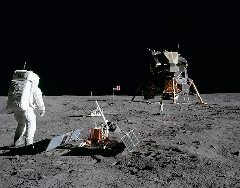
Astronaut Buzz Aldrin on the moon during the Apollo 11 mission. Image via Neil Armstrong/NASA.

Jean Creighton, University of Wisconsin-Milwaukee

Much of the technology common in daily life today originates from the drive to put a human being on the moon. This effort reached its pinnacle when Neil Armstrong stepped off the Eagle landing module onto the lunar surface 50 years ago.

As a NASA airborne astronomy ambassador and director of the University of Wisconsin-Milwaukee Manfred Olson Planetarium, I know that the technologies behind weather forecasting, GPS and even smartphones can trace their origins to the race to the moon.

A Saturn V rocket carrying Apollo 11 and its crew toward the moon lifts off on July 16, 1969. Image via NASA.

1. Rockets

October 4, 1957 marked the dawn of the Space Age, when the Soviet Union launched Sputnik 1, the first human-made satellite. The Soviets were the first to make powerful launch vehicles by adapting World War II-era long-range missiles, especially the German V-2.

From there, space propulsion and satellite technology moved fast: Luna 1 escaped the Earth’s gravitational field to fly past the moon on January 4, 1959; Vostok 1 carried the first human, Yuri Gagarin, into space on April 12, 1961; and Telstar, the first commercial satellite, sent TV signals across the Atlantic Ocean on July 10, 1962.

The 1969 lunar landing also harnessed the expertise of German scientists, such as Wernher von Braun, to send massive payloads into space. The F-1 engines in Saturn V, the Apollo program’s launch vehicle, burned a total of 2,800 tons of fuel at a rate of 12.9 tons per second.

Saturn V still stands as the most powerful rocket ever built, but rockets today are far cheaper to launch. For example, whereas Saturn V cost US$185 million, which translates into over $1 billion in 2019, today’s Falcon Heavy launch costs only $90 million. Those rockets are how satellites, astronauts and other spacecraft get off the Earth’s surface, to continue bringing back information and insights from other worlds.

2. Satellites

The quest for enough thrust to land a man on the moon led to the building of vehicles powerful enough to launch payloads to heights of 21,200 to 22,600 miles (34,100 to 36,440 km) above the Earth’s surface. At such altitudes, satellites’ orbiting speed aligns with how fast the planet spins – so satellites remain over a fixed point, in what is called geosynchronous orbit. Geosynchronous satellites are responsible for communications, providing both internet connectivity and TV programming.

At the beginning of 2019, there were 4,987 satellites orbiting Earth; in 2018 alone, there were more than 382 orbital launches worldwide. Of the currently operational satellites, approximately 40% of payloads enable communications, 36% observe the Earth, 11% demonstrate technologies, 7% improve navigation and positioning and 6% advance space and earth science.

The Apollo Guidance Computer next to a laptop computer. Image via Autopilot/Wikimedia Commons.

3. Miniaturization

Space missions – back then and even today – have strict limits on how big and how heavy their equipment can be, because so much energy is required to lift off and achieve orbit. These constraints pushed the space industry to find ways to make smaller and lighter versions of almost everything: Even the walls of the lunar landing module were reduced to the thickness of two sheets of paper.

From the late 1940s to the late 1960s, the weight and energy consumption of electronics was reduced by a factor of several hundred at least – from the 30 tons and 160 kilowatts of the Electric Numerical Integrator and Computer to the 70 pounds and 70 watts of the Apollo guidance computer. This weight difference is equivalent to that between a humpback whale and an armadillo.

Manned missions required more complex systems than earlier, unmanned ones. For example, in 1951, the Universal Automatic Computer was capable of 1,905 instructions per second, whereas the Saturn V’s guidance system performed 12,190 instructions per second. The trend toward nimble electronics has continued, with modern hand-held devices routinely capable of performing instructions 120 million times faster than the guidance system that enabled the liftoff of Apollo 11. The need to miniaturize computers for space exploration in the 1960s motivated the entire industry to design smaller, faster and more energy-efficient computers, which have affected practically every facet of life today, from communications to health and from manufacturing to transportation.

4. Global network of ground stations

Communicating with vehicles and people in space was just as important as getting them up there in the first place. An important breakthrough associated with the 1969 lunar landing was the construction of a global network of ground stations, called the Deep Space Network, to let controllers on Earth communicate constantly with missions in highly elliptical Earth orbits or beyond. This continuity was possible because the ground facilities were placed strategically 120 degrees apart in longitude so that each spacecraft would be in range of one of the ground stations at all times.

Because of the spacecraft’s limited power capacity, large antennas were built on Earth to simulate “big ears” to hear weak messages and to act as “big mouths” to broadcast loud commands. In fact, the Deep Space Network was used to communicate with the astronauts on Apollo 11 and was used to relay the first dramatic TV images of Neil Armstrong stepping onto the moon. The network was also critical for the survival of the crew on Apollo 13 because they needed guidance from ground personnel without wasting their precious power on communications.

Several dozen missions use the Deep Space Network as part of the continuing exploration of our solar system and beyond. In addition, the Deep Space Network permits communications with satellites that are on highly elliptical orbits, to monitor the poles and deliver radio signals.

‘Earthrise,’ a view of Earth while orbiting the moon. Image via Bill Anders, Apollo 8/NASA

5. Looking back at Earth

Getting to space has allowed people to turn their research efforts toward Earth. In August 1959, the unmanned satellite Explorer VI took the first crude photos of Earth from space on a mission researching the upper atmosphere, in preparation for the Apollo program.

Almost a decade later, the crew of Apollo 8 took a famous picture of the Earth rising over the lunar landscape, aptly named “Earthrise.” This image helped people understand our planet as a unique shared world and boosted the environmental movement.

Earth from the edge of the solar system, visible as a minuscule pale blue dot in the center of the right-most brown stripe. Image via Voyager 1/NASA/

Understanding of our planet’s role in the universe deepened with Voyager 1’s “pale blue dot” photo – an image received by the Deep Space Network.

People and our machines have been taking pictures of the Earth from space ever since. Views of Earth from space guide people both globally and locally. What started in the early 1960s as a U.S. Navy satellite system to track its Polaris submarines to within 600 feet (185 meters) has blossomed into the Global Positioning System network of satellites providing location services worldwide.

Images from a series of Earth-observing satellites called Landsat are used to determine crop health, identify algae blooms and find potential oil deposits. Other uses include identifying which types of forest management are most effective in slowing the spread of wildfires or recognizing global changes such as glacier coverage and urban development.

As we learn more about our own planet and about exoplanets – planets around other stars – we become more aware of how precious our planet is. Efforts to preserve Earth itself may yet find help from fuel cells, another technology from the Apollo program. These storage systems for hydrogen and oxygen in the Apollo Service Module, which contained life-support systems and supplies for the lunar landing missions, generated power and produced potable water for the astronauts. Much cleaner energy sources than traditional combustion engines, fuel cells may play a part in transforming global energy production to fight climate change.

We can only wonder what innovations from the effort to send people to other planets will affect earthlings 50 years after the first Marswalk.

Jean Creighton, Planetarium Director, NASA Airborne Astronomy Ambassador, University of Wisconsin-Milwaukee

This article is republished from The Conversation under a Creative Commons license. Read the original article.

Bottom line: Apollo 11 moon-landing innovations that changed life on Earth.

from EarthSky https://ift.tt/32MgzFo

Astronaut Buzz Aldrin on the moon during the Apollo 11 mission. Image via Neil Armstrong/NASA.

Jean Creighton, University of Wisconsin-Milwaukee

Much of the technology common in daily life today originates from the drive to put a human being on the moon. This effort reached its pinnacle when Neil Armstrong stepped off the Eagle landing module onto the lunar surface 50 years ago.

As a NASA airborne astronomy ambassador and director of the University of Wisconsin-Milwaukee Manfred Olson Planetarium, I know that the technologies behind weather forecasting, GPS and even smartphones can trace their origins to the race to the moon.

A Saturn V rocket carrying Apollo 11 and its crew toward the moon lifts off on July 16, 1969. Image via NASA.

1. Rockets

October 4, 1957 marked the dawn of the Space Age, when the Soviet Union launched Sputnik 1, the first human-made satellite. The Soviets were the first to make powerful launch vehicles by adapting World War II-era long-range missiles, especially the German V-2.

From there, space propulsion and satellite technology moved fast: Luna 1 escaped the Earth’s gravitational field to fly past the moon on January 4, 1959; Vostok 1 carried the first human, Yuri Gagarin, into space on April 12, 1961; and Telstar, the first commercial satellite, sent TV signals across the Atlantic Ocean on July 10, 1962.

The 1969 lunar landing also harnessed the expertise of German scientists, such as Wernher von Braun, to send massive payloads into space. The F-1 engines in Saturn V, the Apollo program’s launch vehicle, burned a total of 2,800 tons of fuel at a rate of 12.9 tons per second.

Saturn V still stands as the most powerful rocket ever built, but rockets today are far cheaper to launch. For example, whereas Saturn V cost US$185 million, which translates into over $1 billion in 2019, today’s Falcon Heavy launch costs only $90 million. Those rockets are how satellites, astronauts and other spacecraft get off the Earth’s surface, to continue bringing back information and insights from other worlds.

2. Satellites

The quest for enough thrust to land a man on the moon led to the building of vehicles powerful enough to launch payloads to heights of 21,200 to 22,600 miles (34,100 to 36,440 km) above the Earth’s surface. At such altitudes, satellites’ orbiting speed aligns with how fast the planet spins – so satellites remain over a fixed point, in what is called geosynchronous orbit. Geosynchronous satellites are responsible for communications, providing both internet connectivity and TV programming.

At the beginning of 2019, there were 4,987 satellites orbiting Earth; in 2018 alone, there were more than 382 orbital launches worldwide. Of the currently operational satellites, approximately 40% of payloads enable communications, 36% observe the Earth, 11% demonstrate technologies, 7% improve navigation and positioning and 6% advance space and earth science.

The Apollo Guidance Computer next to a laptop computer. Image via Autopilot/Wikimedia Commons.

3. Miniaturization

Space missions – back then and even today – have strict limits on how big and how heavy their equipment can be, because so much energy is required to lift off and achieve orbit. These constraints pushed the space industry to find ways to make smaller and lighter versions of almost everything: Even the walls of the lunar landing module were reduced to the thickness of two sheets of paper.

From the late 1940s to the late 1960s, the weight and energy consumption of electronics was reduced by a factor of several hundred at least – from the 30 tons and 160 kilowatts of the Electric Numerical Integrator and Computer to the 70 pounds and 70 watts of the Apollo guidance computer. This weight difference is equivalent to that between a humpback whale and an armadillo.

Manned missions required more complex systems than earlier, unmanned ones. For example, in 1951, the Universal Automatic Computer was capable of 1,905 instructions per second, whereas the Saturn V’s guidance system performed 12,190 instructions per second. The trend toward nimble electronics has continued, with modern hand-held devices routinely capable of performing instructions 120 million times faster than the guidance system that enabled the liftoff of Apollo 11. The need to miniaturize computers for space exploration in the 1960s motivated the entire industry to design smaller, faster and more energy-efficient computers, which have affected practically every facet of life today, from communications to health and from manufacturing to transportation.

4. Global network of ground stations

Communicating with vehicles and people in space was just as important as getting them up there in the first place. An important breakthrough associated with the 1969 lunar landing was the construction of a global network of ground stations, called the Deep Space Network, to let controllers on Earth communicate constantly with missions in highly elliptical Earth orbits or beyond. This continuity was possible because the ground facilities were placed strategically 120 degrees apart in longitude so that each spacecraft would be in range of one of the ground stations at all times.

Because of the spacecraft’s limited power capacity, large antennas were built on Earth to simulate “big ears” to hear weak messages and to act as “big mouths” to broadcast loud commands. In fact, the Deep Space Network was used to communicate with the astronauts on Apollo 11 and was used to relay the first dramatic TV images of Neil Armstrong stepping onto the moon. The network was also critical for the survival of the crew on Apollo 13 because they needed guidance from ground personnel without wasting their precious power on communications.

Several dozen missions use the Deep Space Network as part of the continuing exploration of our solar system and beyond. In addition, the Deep Space Network permits communications with satellites that are on highly elliptical orbits, to monitor the poles and deliver radio signals.

‘Earthrise,’ a view of Earth while orbiting the moon. Image via Bill Anders, Apollo 8/NASA

5. Looking back at Earth

Getting to space has allowed people to turn their research efforts toward Earth. In August 1959, the unmanned satellite Explorer VI took the first crude photos of Earth from space on a mission researching the upper atmosphere, in preparation for the Apollo program.

Almost a decade later, the crew of Apollo 8 took a famous picture of the Earth rising over the lunar landscape, aptly named “Earthrise.” This image helped people understand our planet as a unique shared world and boosted the environmental movement.

Earth from the edge of the solar system, visible as a minuscule pale blue dot in the center of the right-most brown stripe. Image via Voyager 1/NASA/

Understanding of our planet’s role in the universe deepened with Voyager 1’s “pale blue dot” photo – an image received by the Deep Space Network.

People and our machines have been taking pictures of the Earth from space ever since. Views of Earth from space guide people both globally and locally. What started in the early 1960s as a U.S. Navy satellite system to track its Polaris submarines to within 600 feet (185 meters) has blossomed into the Global Positioning System network of satellites providing location services worldwide.

Images from a series of Earth-observing satellites called Landsat are used to determine crop health, identify algae blooms and find potential oil deposits. Other uses include identifying which types of forest management are most effective in slowing the spread of wildfires or recognizing global changes such as glacier coverage and urban development.

As we learn more about our own planet and about exoplanets – planets around other stars – we become more aware of how precious our planet is. Efforts to preserve Earth itself may yet find help from fuel cells, another technology from the Apollo program. These storage systems for hydrogen and oxygen in the Apollo Service Module, which contained life-support systems and supplies for the lunar landing missions, generated power and produced potable water for the astronauts. Much cleaner energy sources than traditional combustion engines, fuel cells may play a part in transforming global energy production to fight climate change.

We can only wonder what innovations from the effort to send people to other planets will affect earthlings 50 years after the first Marswalk.

Jean Creighton, Planetarium Director, NASA Airborne Astronomy Ambassador, University of Wisconsin-Milwaukee

This article is republished from The Conversation under a Creative Commons license. Read the original article.

Bottom line: Apollo 11 moon-landing innovations that changed life on Earth.

from EarthSky https://ift.tt/32MgzFo

Vega and its constellation Lyra

Tonight, look eastward during the evening hours, and it’s hard to miss the season’s signature star formation, called the Summer Triangle. Its stars – Vega, Deneb and Altair – are the first three to light up the eastern half of sky after sunset, and their bright and sparkling radiance is even visible from light-polluted cities or on a moonlit night.

Try looking first for the most prominent star in the eastern sky, which is Vega in the constellation Lyra the Harp. Vega is blue-white in color. It’s sometimes called the Harp Star. And many people recognize its constellation, Lyra, as a triangle of stars connected to a parallelogram.

The constellation Lyra the Harp.

It’s hard to gauge the humongous size of the Summer Triangle by looking at our little chart. A 12-inch ruler, when placed at an arm’s length from your eye, spans the approximate distance from Vega to the star Altair. And an outstretched hand more or less fills the gap between Vega and Deneb.

More than any other month, July is the month of the Summer Triangle. At mid-northern latitudes, the Summer Triangle’s stars – as if a trio of school kids on vacation – stay out from dusk till dawn, dancing amid the stars of our Milky Way galaxy. As our Earth turns tonight, Vega, Deneb and Altair travel westward across the sky. The Summer Triangle shines high overhead in the middle of the night, and sparkles in the west as the rose-colored dawn begins to color the sky.

The Summer Triangle, photographed by Susan Jensen in Odessa, Washington.

Our Summer Triangle series also includes:

Part 2: Deneb and its constellation Cygnus

Part 3: Altair and its constellation Aquila

EarthSky astronomy kits are perfect for beginners. Order yours today.

Bottom line: The Summer Triangle consists of 3 bright stars in 3 different constellations. The brightest is Vega in the constellation Lyra.

from EarthSky https://ift.tt/2LtdODm

Tonight, look eastward during the evening hours, and it’s hard to miss the season’s signature star formation, called the Summer Triangle. Its stars – Vega, Deneb and Altair – are the first three to light up the eastern half of sky after sunset, and their bright and sparkling radiance is even visible from light-polluted cities or on a moonlit night.

Try looking first for the most prominent star in the eastern sky, which is Vega in the constellation Lyra the Harp. Vega is blue-white in color. It’s sometimes called the Harp Star. And many people recognize its constellation, Lyra, as a triangle of stars connected to a parallelogram.

The constellation Lyra the Harp.

It’s hard to gauge the humongous size of the Summer Triangle by looking at our little chart. A 12-inch ruler, when placed at an arm’s length from your eye, spans the approximate distance from Vega to the star Altair. And an outstretched hand more or less fills the gap between Vega and Deneb.

More than any other month, July is the month of the Summer Triangle. At mid-northern latitudes, the Summer Triangle’s stars – as if a trio of school kids on vacation – stay out from dusk till dawn, dancing amid the stars of our Milky Way galaxy. As our Earth turns tonight, Vega, Deneb and Altair travel westward across the sky. The Summer Triangle shines high overhead in the middle of the night, and sparkles in the west as the rose-colored dawn begins to color the sky.

The Summer Triangle, photographed by Susan Jensen in Odessa, Washington.

Our Summer Triangle series also includes:

Part 2: Deneb and its constellation Cygnus

Part 3: Altair and its constellation Aquila

EarthSky astronomy kits are perfect for beginners. Order yours today.

Bottom line: The Summer Triangle consists of 3 bright stars in 3 different constellations. The brightest is Vega in the constellation Lyra.

from EarthSky https://ift.tt/2LtdODm

What will Earth’s next supercontinent look like?

Planet Earth. Image via Triff/Shutterstock

Over geologic timescales, Earth’s continents continually change. Geologists believe that, every few hundred million years, the continents combine to create massive supercontinents. The most famous past supercontinent is probably the most recent one, Pangea. This article on future supercontinents was originally published November 27, 2018. EarthSky blogger Deanna Conners brought it to our attention last week, and we couldn’t resist it. It gives 4 possible scenarios describing what our planet might look like when the next supercontinent forms.

By Mattias Green, Bangor University; Hannah Sophia Davies, Universidade de Lisboa , and Joao C. Duarte, Universidade de Lisboa

The outer layer of the Earth, the solid crust we walk on, is made up of broken pieces, much like the shell of a broken egg. These pieces, the tectonic plates, move around the planet at speeds of a few centimeters per year. Every so often they come together and combine into a supercontinent, which remains for a few hundred million years before breaking up. The plates then disperse or scatter and move away from each other, until they eventually – after another 400-600 million years – come back together again.

The last supercontinent, Pangea, formed around 310 million years ago, and started breaking up around 180 million years ago. It has been suggested that the next supercontinent will form in 200-250 million years, so we are currently about halfway through the scattered phase of the current supercontinent cycle. The question is: how will the next supercontinent form, and why?

There are four fundamental scenarios for the formation of the next supercontinent: Novopangea, Pangea Ultima, Aurica and Amasia. How each forms depends on different scenarios but ultimately are linked to how Pangea separated, and how the world’s continents are still moving today.

The breakup of Pangea led to the formation of the Atlantic Ocean, which is still opening and getting wider today. Consequently, the Pacific Ocean is closing and getting narrower. The Pacific is home to a ring of subduction zones along its edges (the “ring of fire”), where ocean floor is brought down, or subducted, under continental plates and into the Earth’s interior. There, the old ocean floor is recycled and can go into volcanic plumes. The Atlantic, by contrast, has a large ocean ridge producing new ocean plate, but is only home to two subduction zones: the Lesser Antilles Arc in the Caribbean and the Scotia Arc between South America and Antarctica.

1. Novopangea

If we assume that present day conditions persist, so that the Atlantic continues to open and the Pacific keeps closing, we have a scenario where the next supercontinent forms in the antipodes of Pangea. The Americas would collide with the northward drifting Antarctica, and then into the already collided Africa-Eurasia. The supercontinent that would then form has been named Novopangea, or Novopangaea.

Novopangea.

2. Pangea Ultima

The Atlantic opening may, however, slow down and actually start closing in the future. The two small arcs of subduction in the Atlantic could potentially spread all along the east coasts of the Americas, leading to a reforming of Pangea as the Americas, Europe and Africa are brought back together into a supercontinent called Pangea Ultima. This new supercontinent would be surrounded by a super Pacific Ocean.

Pangea Ultima, formed by the Atlantic closing.

3. Aurica

However, if the Atlantic was to develop new subduction zones – something that may already be happening – both the Pacific and Atlantic oceans may be fated to close. This means that a a new ocean basin would have to form to replace them.

In this scenario the Pan-Asian rift currently cutting through Asia from west of India up to the Arctic opens to form the new ocean. The result is the formation of the supercontinent Aurica. Because of Australia’s current northwards drift it would be at the center of the new continent as East Asia and the Americas close the Pacific from either side. The European and African plates would then rejoin the Americas as the Atlantic closes.

4. Amasia

The fourth scenario predicts a completely different fate for future Earth. Several of the tectonic plates are currently moving north, including both Africa and Australia. This drift is believed to be driven by anomalies left by Pangea, deep in the Earth’s interior, in the part called the mantle. Because of this northern drift, one can envisage a scenario where the continents, except Antarctica, keep drifting north. This means that they would eventually gather around the North Pole in a supercontinent called Amasia. In this scenario, both the Atlantic and the Pacific would mostly remain open.

Amasia, the fourth scenario.

Of these four scenarios we believe that Novopangea is the most likely. It is a logical progression of present day continental plate drift directions, while the other three assume that another process comes into play. There would need to be new Atlantic subduction zones for Aurica, the reversal of the Atlantic opening for Pangea Ultima, or anomalies in the Earth’s interior left by Pangea for Amasia.

Investigating the Earth’s tectonic future forces us to push the boundaries of our knowledge, and to think about the processes that shape our planet over long time scales. It also leads us to think about the Earth system as a whole, and raises a series of other questions – what will the climate of the next supercontinent be? How will the ocean circulation adjust? How will life evolve and adapt? These are the kind of questions that push the boundaries of science further because they push the boundaries of our imagination.

Mattias Green, Reader in Physical Oceanography, Bangor University; Hannah Sophia Davies, Ph.D. Researcher, Universidade de Lisboa, and Joao C. Duarte, Researcher and Coordinator of the Marine Geology and Geophysics Group, Universidade de Lisboa

This article is republished from The Conversation under a Creative Commons license. Read the original article.

Bottom line: What planet Earth might look like when the next supercontinent forms – four scenarios.

from EarthSky https://ift.tt/2Y9aUcW

Planet Earth. Image via Triff/Shutterstock

Over geologic timescales, Earth’s continents continually change. Geologists believe that, every few hundred million years, the continents combine to create massive supercontinents. The most famous past supercontinent is probably the most recent one, Pangea. This article on future supercontinents was originally published November 27, 2018. EarthSky blogger Deanna Conners brought it to our attention last week, and we couldn’t resist it. It gives 4 possible scenarios describing what our planet might look like when the next supercontinent forms.

By Mattias Green, Bangor University; Hannah Sophia Davies, Universidade de Lisboa , and Joao C. Duarte, Universidade de Lisboa

The outer layer of the Earth, the solid crust we walk on, is made up of broken pieces, much like the shell of a broken egg. These pieces, the tectonic plates, move around the planet at speeds of a few centimeters per year. Every so often they come together and combine into a supercontinent, which remains for a few hundred million years before breaking up. The plates then disperse or scatter and move away from each other, until they eventually – after another 400-600 million years – come back together again.

The last supercontinent, Pangea, formed around 310 million years ago, and started breaking up around 180 million years ago. It has been suggested that the next supercontinent will form in 200-250 million years, so we are currently about halfway through the scattered phase of the current supercontinent cycle. The question is: how will the next supercontinent form, and why?

There are four fundamental scenarios for the formation of the next supercontinent: Novopangea, Pangea Ultima, Aurica and Amasia. How each forms depends on different scenarios but ultimately are linked to how Pangea separated, and how the world’s continents are still moving today.

The breakup of Pangea led to the formation of the Atlantic Ocean, which is still opening and getting wider today. Consequently, the Pacific Ocean is closing and getting narrower. The Pacific is home to a ring of subduction zones along its edges (the “ring of fire”), where ocean floor is brought down, or subducted, under continental plates and into the Earth’s interior. There, the old ocean floor is recycled and can go into volcanic plumes. The Atlantic, by contrast, has a large ocean ridge producing new ocean plate, but is only home to two subduction zones: the Lesser Antilles Arc in the Caribbean and the Scotia Arc between South America and Antarctica.

1. Novopangea

If we assume that present day conditions persist, so that the Atlantic continues to open and the Pacific keeps closing, we have a scenario where the next supercontinent forms in the antipodes of Pangea. The Americas would collide with the northward drifting Antarctica, and then into the already collided Africa-Eurasia. The supercontinent that would then form has been named Novopangea, or Novopangaea.

Novopangea.

2. Pangea Ultima

The Atlantic opening may, however, slow down and actually start closing in the future. The two small arcs of subduction in the Atlantic could potentially spread all along the east coasts of the Americas, leading to a reforming of Pangea as the Americas, Europe and Africa are brought back together into a supercontinent called Pangea Ultima. This new supercontinent would be surrounded by a super Pacific Ocean.

Pangea Ultima, formed by the Atlantic closing.

3. Aurica

However, if the Atlantic was to develop new subduction zones – something that may already be happening – both the Pacific and Atlantic oceans may be fated to close. This means that a a new ocean basin would have to form to replace them.

In this scenario the Pan-Asian rift currently cutting through Asia from west of India up to the Arctic opens to form the new ocean. The result is the formation of the supercontinent Aurica. Because of Australia’s current northwards drift it would be at the center of the new continent as East Asia and the Americas close the Pacific from either side. The European and African plates would then rejoin the Americas as the Atlantic closes.

4. Amasia

The fourth scenario predicts a completely different fate for future Earth. Several of the tectonic plates are currently moving north, including both Africa and Australia. This drift is believed to be driven by anomalies left by Pangea, deep in the Earth’s interior, in the part called the mantle. Because of this northern drift, one can envisage a scenario where the continents, except Antarctica, keep drifting north. This means that they would eventually gather around the North Pole in a supercontinent called Amasia. In this scenario, both the Atlantic and the Pacific would mostly remain open.

Amasia, the fourth scenario.

Of these four scenarios we believe that Novopangea is the most likely. It is a logical progression of present day continental plate drift directions, while the other three assume that another process comes into play. There would need to be new Atlantic subduction zones for Aurica, the reversal of the Atlantic opening for Pangea Ultima, or anomalies in the Earth’s interior left by Pangea for Amasia.

Investigating the Earth’s tectonic future forces us to push the boundaries of our knowledge, and to think about the processes that shape our planet over long time scales. It also leads us to think about the Earth system as a whole, and raises a series of other questions – what will the climate of the next supercontinent be? How will the ocean circulation adjust? How will life evolve and adapt? These are the kind of questions that push the boundaries of science further because they push the boundaries of our imagination.

Mattias Green, Reader in Physical Oceanography, Bangor University; Hannah Sophia Davies, Ph.D. Researcher, Universidade de Lisboa, and Joao C. Duarte, Researcher and Coordinator of the Marine Geology and Geophysics Group, Universidade de Lisboa

This article is republished from The Conversation under a Creative Commons license. Read the original article.

Bottom line: What planet Earth might look like when the next supercontinent forms – four scenarios.

from EarthSky https://ift.tt/2Y9aUcW

Ancient hyenas roamed the Arctic

An artist’s rendering of ancient Arctic hyenas. Image via Julius T. Csotonyi/University of Buffalo.

A new study reports that two enigmatic fossil teeth found in Yukon Territory in Canada in the 1970s belonged to an extinct hyena, the so-called “running hyena” or Chasmaporthetes.

Modern hyenas are hunters and scavengers in the Asian and African savannas. But the study, published June 18, 2019, in the peer-reviewed journal Open Quaternary, reveals that during the last ice age these powerful carnivores also roamed the frigid Arctic.

Government of Yukon paleontologist Grant Zazula is a study co-author. He said in a statement:

It is amazing to imagine hyenas thriving in the harsh conditions above the Arctic Circle during the ice age. Chasmaporthetes probably hunted herds of ice age caribou and horses or scavenged carcasses of mammoths on the vast steppe-tundra that stretched from Siberia to Yukon Territory.

The findings fill an important gap in scientists’ knowledge of how hyenas reached North America. Previously, Chasmaporthetes fossils had been found as far north as Mongolia in Asia and the southern United States in North America, with no sites in between. University of Buffalo paleontologist Jack Tseng is the paper’s first author. Tseng said:

Fossils of this genus of hyenas had been found in Africa, Europe and Asia, and also in the southern United States. But where and how did these animals get to North America? The teeth we studied, even though they were just two teeth, start to answer those questions.

This ice age fossil tooth – tucked away for years in the collections of the Canadian Museum of Nature – belonged to the “running hyena” Chasmaporthetes, according to a new University at Buffalo-led study. This tooth, found in 1977, and one other are the first known hyena fossils found in the Arctic. Image via Grant Zazula/Government of Yukon.

According to the researchers, ancient hyenas likely entered North America via Beringia, an area, including Alaska and Yukon Territory, that connects Asia with North America during periods of low sea levels. From there, the animals made their way south all the way to Mexico, scientists say. The newly-described fossils provide the first proof of ancient hyenas living in Beringia. Tseng said:

Our previous understanding of where these far-ranging hyenas lived was based on fossil records in southern North America on one hand, and Asia, Europe and Africa on the other. These rare records of hyenas in the Arctic fill in a massive gap in a location where we expected evidence of their crossing between continents, but had no proof until now.

The fossil teeth are most likely between about 1.4 million and 850,000 years old, according to the researchers’ analysis. But the first hyenas crossed into North America long before that, says Tseng, as the earliest known hyena fossils on the continent date back about 5 million years.

The fossil teeth were collected in the 1970s during paleontological expeditions in the remote Old Crow River region (Vuntut Gwitchin First Nation) in northern Yukon Territory, an area known for its rich deposits of fossils. The ancient hyena teeth are among 50,000 fossils recovered from the region in the last century. Image via Duane Froese/University of Alberta.

Though there are four living species of hyena today (three bone-crushing species, plus the ant-eating aardwolf), hyenas disappeared from North America before the first people arrived. Although the reasons for this extinction between 1 and 0.5 million years ago remain unclear, it is possible that the animals’ bone-crushing, scavenging niche was replaced by the impressive short-faced bear, which lived across North America until the end of the ice age about 12,000 years ago.

Bottom line: Fossil teeth suggest ancient hyenas roamed the Arctic.

Source: First Fossils of Hyenas (Chasmaporthetes, Hyaenidae, Carnivora) from North of the Arctic Circle

Via University of Buffalo

from EarthSky https://ift.tt/2SlbzCJ

An artist’s rendering of ancient Arctic hyenas. Image via Julius T. Csotonyi/University of Buffalo.

A new study reports that two enigmatic fossil teeth found in Yukon Territory in Canada in the 1970s belonged to an extinct hyena, the so-called “running hyena” or Chasmaporthetes.

Modern hyenas are hunters and scavengers in the Asian and African savannas. But the study, published June 18, 2019, in the peer-reviewed journal Open Quaternary, reveals that during the last ice age these powerful carnivores also roamed the frigid Arctic.

Government of Yukon paleontologist Grant Zazula is a study co-author. He said in a statement:

It is amazing to imagine hyenas thriving in the harsh conditions above the Arctic Circle during the ice age. Chasmaporthetes probably hunted herds of ice age caribou and horses or scavenged carcasses of mammoths on the vast steppe-tundra that stretched from Siberia to Yukon Territory.

The findings fill an important gap in scientists’ knowledge of how hyenas reached North America. Previously, Chasmaporthetes fossils had been found as far north as Mongolia in Asia and the southern United States in North America, with no sites in between. University of Buffalo paleontologist Jack Tseng is the paper’s first author. Tseng said:

Fossils of this genus of hyenas had been found in Africa, Europe and Asia, and also in the southern United States. But where and how did these animals get to North America? The teeth we studied, even though they were just two teeth, start to answer those questions.

This ice age fossil tooth – tucked away for years in the collections of the Canadian Museum of Nature – belonged to the “running hyena” Chasmaporthetes, according to a new University at Buffalo-led study. This tooth, found in 1977, and one other are the first known hyena fossils found in the Arctic. Image via Grant Zazula/Government of Yukon.

According to the researchers, ancient hyenas likely entered North America via Beringia, an area, including Alaska and Yukon Territory, that connects Asia with North America during periods of low sea levels. From there, the animals made their way south all the way to Mexico, scientists say. The newly-described fossils provide the first proof of ancient hyenas living in Beringia. Tseng said:

Our previous understanding of where these far-ranging hyenas lived was based on fossil records in southern North America on one hand, and Asia, Europe and Africa on the other. These rare records of hyenas in the Arctic fill in a massive gap in a location where we expected evidence of their crossing between continents, but had no proof until now.

The fossil teeth are most likely between about 1.4 million and 850,000 years old, according to the researchers’ analysis. But the first hyenas crossed into North America long before that, says Tseng, as the earliest known hyena fossils on the continent date back about 5 million years.

The fossil teeth were collected in the 1970s during paleontological expeditions in the remote Old Crow River region (Vuntut Gwitchin First Nation) in northern Yukon Territory, an area known for its rich deposits of fossils. The ancient hyena teeth are among 50,000 fossils recovered from the region in the last century. Image via Duane Froese/University of Alberta.

Though there are four living species of hyena today (three bone-crushing species, plus the ant-eating aardwolf), hyenas disappeared from North America before the first people arrived. Although the reasons for this extinction between 1 and 0.5 million years ago remain unclear, it is possible that the animals’ bone-crushing, scavenging niche was replaced by the impressive short-faced bear, which lived across North America until the end of the ice age about 12,000 years ago.

Bottom line: Fossil teeth suggest ancient hyenas roamed the Arctic.

Source: First Fossils of Hyenas (Chasmaporthetes, Hyaenidae, Carnivora) from North of the Arctic Circle

Via University of Buffalo

from EarthSky https://ift.tt/2SlbzCJ

Watch for a daytime moon

In the coming mornings, watch for a daytime moon. No matter where you are on Earth, look generally westward after sunrise to see the moon in a blue daytime sky, assuming yours is clear.

Why can you see the moon in the daytime now? The full moon – and partial lunar eclipse – happened during the night of Tuesday, July 16, 2019 (or the morning of Wednesday, July 17, for some). In the days after full moon, the moon is officially in a waning gibbous phase, rising after nightfall and setting in a westward direction shortly after sunrise.

July 29, 2018, daytime moon – caught from a rooftop in New York City – via our friend Ben Orlove.

If you look for the moon at the same time every morning, you’ll see this week’s waning moon appearing higher and higher in the western sky each early morning, for several days. To understand why, think about where the sun is in early morning. A full moon is opposite the sun, in the west when the sun is in the east. Except now it’s after full moon. The moon is moving in its orbit around Earth – moving toward the east, as it always does – drawing closer and closer to the Earth-sun line.

By July 25, 2019, the moon will be at the last quarter phase – rising around midnight and southward around dawn. Then the moon will turn new again on August 1. It’ll be rising and setting with the sun, giving us deliciously dark skies for the upcoming Delta Aquariid meteor shower, plus a waxing crescent moon in early August, when the annual Perseid meteor shower is rising to its peak.

People love to see the daytime moon. They wonder about it, and ask about it. Once, a reader in Kansas City wrote in with the name children’s moon to describe a moon visible during the day. She said this name stemmed from the idea that children can’t stay up at night late enough to see the moon when it appears only in darkness.

That story prompted another reader to send in an alternate version for the origin of the name children’s moon. She wrote:

I heard a daytime moon was called a ‘children’s moon’ because their eyes were sharp enough to pick it out, where the old folks, with fading vision, could not tell it from the clouds.

Can you see the daytime moon in the next few mornings?

Here’s another July daytime moon – from the year 2017 – from Jeff Hagan in Yakima, Washington. He wrote: “I woke up early and stepped onto the deck at our house in Yakima to check the weather. I was just in time to watch the full moon set over Mt. Adams, a 12,300-foot glaciated volcano in the Cascade Mountains. The moon appeared to be rolling down the north ridge of the mountain.”

Bottom line: In the days after every full moon, the moon appears in the west after sunrise, in a blue sky. Watch for it.

A planisphere is virtually indispensable for beginning stargazers. Order your EarthSky planisphere today.

Four keys to understanding moon phases

from EarthSky https://ift.tt/2YWMpNl

In the coming mornings, watch for a daytime moon. No matter where you are on Earth, look generally westward after sunrise to see the moon in a blue daytime sky, assuming yours is clear.

Why can you see the moon in the daytime now? The full moon – and partial lunar eclipse – happened during the night of Tuesday, July 16, 2019 (or the morning of Wednesday, July 17, for some). In the days after full moon, the moon is officially in a waning gibbous phase, rising after nightfall and setting in a westward direction shortly after sunrise.

July 29, 2018, daytime moon – caught from a rooftop in New York City – via our friend Ben Orlove.

If you look for the moon at the same time every morning, you’ll see this week’s waning moon appearing higher and higher in the western sky each early morning, for several days. To understand why, think about where the sun is in early morning. A full moon is opposite the sun, in the west when the sun is in the east. Except now it’s after full moon. The moon is moving in its orbit around Earth – moving toward the east, as it always does – drawing closer and closer to the Earth-sun line.

By July 25, 2019, the moon will be at the last quarter phase – rising around midnight and southward around dawn. Then the moon will turn new again on August 1. It’ll be rising and setting with the sun, giving us deliciously dark skies for the upcoming Delta Aquariid meteor shower, plus a waxing crescent moon in early August, when the annual Perseid meteor shower is rising to its peak.

People love to see the daytime moon. They wonder about it, and ask about it. Once, a reader in Kansas City wrote in with the name children’s moon to describe a moon visible during the day. She said this name stemmed from the idea that children can’t stay up at night late enough to see the moon when it appears only in darkness.

That story prompted another reader to send in an alternate version for the origin of the name children’s moon. She wrote:

I heard a daytime moon was called a ‘children’s moon’ because their eyes were sharp enough to pick it out, where the old folks, with fading vision, could not tell it from the clouds.

Can you see the daytime moon in the next few mornings?

Here’s another July daytime moon – from the year 2017 – from Jeff Hagan in Yakima, Washington. He wrote: “I woke up early and stepped onto the deck at our house in Yakima to check the weather. I was just in time to watch the full moon set over Mt. Adams, a 12,300-foot glaciated volcano in the Cascade Mountains. The moon appeared to be rolling down the north ridge of the mountain.”

Bottom line: In the days after every full moon, the moon appears in the west after sunrise, in a blue sky. Watch for it.

A planisphere is virtually indispensable for beginning stargazers. Order your EarthSky planisphere today.

Four keys to understanding moon phases

from EarthSky https://ift.tt/2YWMpNl

Enceladus’ ocean right age to support life

The geysers of Saturn’s moon Enceladus. These huge plumes of water vapor erupt through cracks at Enceladus’ south pole. The Cassini spacecraft analyzed the plumes and found they contain water vapor, ice particles, salts, methane and a variety of complex organic molecules. Scientists believe they originate from an ocean below the moon’s icy crust. Image via NASA/JPL-Caltech/Space Science Institute.

Could there be life on Saturn’s moon Enceladus? The moon may be small, but it has a global water ocean beneath its icy surface, and scientists have speculated on whether there is anything alive in that deep, dark abyss. The Cassini spacecraft found that it is salty like oceans on Earth, contains abundant organic molecules, and that there is likely hydrothermal activity on the ocean bottom.

All of those are positive signs for habitability and now scientists have found another one: the ocean appears to be just the right age for optimal life-supporting conditions. The finding was announced by Marc Neveu, a research scientist at NASA’s Goddard Space Flight Center, on June 24, 2019, during a talk at the 2019 Astrobiology Science Conference (AbSciCon2019). The peer-reviewed results had also been previously published April 1, 2019, in the journal Nature Astronomy.

Enceladus’ ocean is now estimated to be 1 billion years old. This is an ideal age, in terms of life starting and evolving. If the ocean were too young, there wouldn’t have been enough time for different elements needed to mix together, but if it were too old, those chemical processes may have stopped already. The moon would’ve then reached a state of equilibrium, meaning that the reactions to sustain life wouldn’t take place any longer.

Enceladus as seen by the Cassini spacecraft. This small, icy moon has a global subsurface ocean that could possibly support life. Image via NASA/JPL-Caltech/NASA Science.

So how did Neveu and his team come to this conclusion? Using data from the Cassini mission, which ended in late 2017, they created 50 different simulations of conditions in Enceladus’ ocean. These included details of Saturn’s moons’ orbits and the radioactivity of the rocks on Enceladus, as well as their own estimates as to the age of the moon and how it formed.

There was one simulation that best re-created the known conditions of the ocean, the one where the ocean is 1 billion years old. Neveu is cautious, though, because the simulation matched most of the conditions, but not all of them:

For example, if you took the present day, the ocean would be refrozen in that simulation which is not what we’re seeing. So the age of the ocean, should be taken with a grain of salt.

As a next step, the researchers want to improve the simulation models, so the ocean can be dated more precisely. As Neveu said:

We want to know this before we go back to search for life.

Illustration depicting the interior of Enceladus. Water from the subsurface ocean percolates to the surface through cracks in the ice at the south pole, erupting in huge plumes. Image via NASA/JPL-Caltech.

The fact that Enceladus has an ocean at all was surprising to planetary scientists, since it is so small and the surface is so cold. According to Neveu:

It’s very surprising to see an ocean today. It’s a very tiny moon and, in general, you expect tiny things to not be very active [but rather] like a dead block of rock and ice.

The Cassini spacecraft studied the composition of the ocean by analyzing the water vapor in the massive plumes that erupt from the moon’s south pole. The plumes originate from the ocean below, where water percolates to the surface through cracks, and then erupts into empty space. Cassini was able to fly right through the plumes, and found they contain water vapor, ice particles, salts, methane and a variety of complex organic molecules.

Cassini also found evidence for current hydrothermal activity – hydrothermal vents – on the ocean floor, just like in oceans on Earth. Such hotspots could provide an oasis of needed heat and energy in the otherwise cold waters. On Earth, similar vents sustain a wide variety of simple life forms. Could the same be true for Enceladus?

The Cassini mission found evidence for hydrothermal activity – hydrothermal vents – on the bottom of Enceladus’ ocean. Could they help sustain life like they do on Earth? Image via NASA/JPL-Caltech/Southwest Research Institute.

Enceladus has all the ingredients considered necessary for life (as we know it at least), and its ocean appears to be quite similar to that of Europa. Whether life of any kind ever actually started here is still unknown, but the prospects seem promising. The only way we can learn more is to go back there with a return mission. None are scheduled yet, but there are mission proposals on the drawing boards, perhaps something similar to the Europa Clipper mission, which is now being designed to launch sometime in the 2020s. That mission will study Europa and its ocean in more detail than ever before, looking for evidence that something might be alive in its dark waters as well.

Bottom line: It turns out that Enceladus’ subsurface ocean is just the right age to support life, according to a new study. Together with what we already know about its potential habitability, this makes Enceladus even more enticing in the search for life elsewhere in the solar system.

Source: Evolution of Saturn’s mid-sized moons

Via Live Science

from EarthSky https://ift.tt/2NWpTD9

The geysers of Saturn’s moon Enceladus. These huge plumes of water vapor erupt through cracks at Enceladus’ south pole. The Cassini spacecraft analyzed the plumes and found they contain water vapor, ice particles, salts, methane and a variety of complex organic molecules. Scientists believe they originate from an ocean below the moon’s icy crust. Image via NASA/JPL-Caltech/Space Science Institute.

Could there be life on Saturn’s moon Enceladus? The moon may be small, but it has a global water ocean beneath its icy surface, and scientists have speculated on whether there is anything alive in that deep, dark abyss. The Cassini spacecraft found that it is salty like oceans on Earth, contains abundant organic molecules, and that there is likely hydrothermal activity on the ocean bottom.

All of those are positive signs for habitability and now scientists have found another one: the ocean appears to be just the right age for optimal life-supporting conditions. The finding was announced by Marc Neveu, a research scientist at NASA’s Goddard Space Flight Center, on June 24, 2019, during a talk at the 2019 Astrobiology Science Conference (AbSciCon2019). The peer-reviewed results had also been previously published April 1, 2019, in the journal Nature Astronomy.

Enceladus’ ocean is now estimated to be 1 billion years old. This is an ideal age, in terms of life starting and evolving. If the ocean were too young, there wouldn’t have been enough time for different elements needed to mix together, but if it were too old, those chemical processes may have stopped already. The moon would’ve then reached a state of equilibrium, meaning that the reactions to sustain life wouldn’t take place any longer.

Enceladus as seen by the Cassini spacecraft. This small, icy moon has a global subsurface ocean that could possibly support life. Image via NASA/JPL-Caltech/NASA Science.

So how did Neveu and his team come to this conclusion? Using data from the Cassini mission, which ended in late 2017, they created 50 different simulations of conditions in Enceladus’ ocean. These included details of Saturn’s moons’ orbits and the radioactivity of the rocks on Enceladus, as well as their own estimates as to the age of the moon and how it formed.

There was one simulation that best re-created the known conditions of the ocean, the one where the ocean is 1 billion years old. Neveu is cautious, though, because the simulation matched most of the conditions, but not all of them:

For example, if you took the present day, the ocean would be refrozen in that simulation which is not what we’re seeing. So the age of the ocean, should be taken with a grain of salt.

As a next step, the researchers want to improve the simulation models, so the ocean can be dated more precisely. As Neveu said:

We want to know this before we go back to search for life.

Illustration depicting the interior of Enceladus. Water from the subsurface ocean percolates to the surface through cracks in the ice at the south pole, erupting in huge plumes. Image via NASA/JPL-Caltech.

The fact that Enceladus has an ocean at all was surprising to planetary scientists, since it is so small and the surface is so cold. According to Neveu:

It’s very surprising to see an ocean today. It’s a very tiny moon and, in general, you expect tiny things to not be very active [but rather] like a dead block of rock and ice.

The Cassini spacecraft studied the composition of the ocean by analyzing the water vapor in the massive plumes that erupt from the moon’s south pole. The plumes originate from the ocean below, where water percolates to the surface through cracks, and then erupts into empty space. Cassini was able to fly right through the plumes, and found they contain water vapor, ice particles, salts, methane and a variety of complex organic molecules.

Cassini also found evidence for current hydrothermal activity – hydrothermal vents – on the ocean floor, just like in oceans on Earth. Such hotspots could provide an oasis of needed heat and energy in the otherwise cold waters. On Earth, similar vents sustain a wide variety of simple life forms. Could the same be true for Enceladus?

The Cassini mission found evidence for hydrothermal activity – hydrothermal vents – on the bottom of Enceladus’ ocean. Could they help sustain life like they do on Earth? Image via NASA/JPL-Caltech/Southwest Research Institute.

Enceladus has all the ingredients considered necessary for life (as we know it at least), and its ocean appears to be quite similar to that of Europa. Whether life of any kind ever actually started here is still unknown, but the prospects seem promising. The only way we can learn more is to go back there with a return mission. None are scheduled yet, but there are mission proposals on the drawing boards, perhaps something similar to the Europa Clipper mission, which is now being designed to launch sometime in the 2020s. That mission will study Europa and its ocean in more detail than ever before, looking for evidence that something might be alive in its dark waters as well.

Bottom line: It turns out that Enceladus’ subsurface ocean is just the right age to support life, according to a new study. Together with what we already know about its potential habitability, this makes Enceladus even more enticing in the search for life elsewhere in the solar system.

Source: Evolution of Saturn’s mid-sized moons

Via Live Science

from EarthSky https://ift.tt/2NWpTD9

Join space scientists marking Apollo anniversary

Astronaut Buzz Aldrin on the moon during the Apollo 11 mission. Image via Neil Armstrong/NASA.

This evening (July 17, 2019), join space scientists at the National Archives in Washington D.C, where they’ll discuss the legacy of Apollo 11, ahead of the mission’s 50th anniversary. Titled Small Steps and Giant Leaps: How Apollo 11 Shaped Our Understanding of Earth and Beyond, the event will highlight how the study of the moon has led to a deeper understanding of Earth and the solar system, including their origins, and what the world stands to learn from continuing planetary science missions.

The program will be streamed live on YouTube, and begins at 7:00 p.m. EDT (23:00 UTC; translate UTC to your time).

Watch here.

Moderated by NASA Chief Scientist Jim Green, the panel will include:

– Sean Solomon, director of the Lamont-Doherty Earth Observatory
– Sonia Tikoo, assistant professor at Stanford University
– Steven Hauck, professor of planetary geodynamics at Case Western Reserve University
– Heather Meyer, postdoctoral fellow at the Lunar and Planetary Institute.

The event is a partnership between the American Geophysical Union (AGU) and the National Archives and as a part of AGU’s Centennial celebration.

Bottom line: Watch leading space scientists discuss the legacy of Apollo 11, ahead of the mission’s 50th anniversary.

from EarthSky https://ift.tt/2XMwKn1

Astronaut Buzz Aldrin on the moon during the Apollo 11 mission. Image via Neil Armstrong/NASA.

This evening (July 17, 2019), join space scientists at the National Archives in Washington D.C, where they’ll discuss the legacy of Apollo 11, ahead of the mission’s 50th anniversary. Titled Small Steps and Giant Leaps: How Apollo 11 Shaped Our Understanding of Earth and Beyond, the event will highlight how the study of the moon has led to a deeper understanding of Earth and the solar system, including their origins, and what the world stands to learn from continuing planetary science missions.

The program will be streamed live on YouTube, and begins at 7:00 p.m. EDT (23:00 UTC; translate UTC to your time).

Watch here.

Moderated by NASA Chief Scientist Jim Green, the panel will include:

– Sean Solomon, director of the Lamont-Doherty Earth Observatory
– Sonia Tikoo, assistant professor at Stanford University
– Steven Hauck, professor of planetary geodynamics at Case Western Reserve University
– Heather Meyer, postdoctoral fellow at the Lunar and Planetary Institute.

The event is a partnership between the American Geophysical Union (AGU) and the National Archives and as a part of AGU’s Centennial celebration.

Bottom line: Watch leading space scientists discuss the legacy of Apollo 11, ahead of the mission’s 50th anniversary.

from EarthSky https://ift.tt/2XMwKn1

Apollo 11 launch pad

View larger. | Image via ESA.

Yesterday (July 16, 2019) the European Space Agency (ESA) released this image to mark 50 years since Apollo 11 blasted off with the first humans to walk on the moon. ESA’s Copernicus Sentinel-2 satellite captured this image of the historic launch site at Kennedy Space Center, Cape Canaveral, Florida, on January 29, 2019.

On July 16, 1969, the Saturn V rocket carrying Apollo 11 began its journey to the moon. It lifted off from launch pad 39A – which is the second pad down from the top in the image. ESA said in an accompanying statement:

The crew – Neil Armstrong, mission commander, Michael Collins, command module pilot and Edwin ‘Buzz’ Aldrin, lunar module pilot – were embarking on a milestone in human history.

Just four days later, the lunar module, the Eagle, touched down. Watched on television by millions around the world, Neil Armstrong was the first to set foot on the moon, famously saying, “That’s one small step for man, one giant leap for mankind.”

Bottom line: Satellite image of Apollo 11 mission launchpad.

Via ESA

from EarthSky https://ift.tt/2ShXsOq

View larger. | Image via ESA.

Yesterday (July 16, 2019) the European Space Agency (ESA) released this image to mark 50 years since Apollo 11 blasted off with the first humans to walk on the moon. ESA’s Copernicus Sentinel-2 satellite captured this image of the historic launch site at Kennedy Space Center, Cape Canaveral, Florida, on January 29, 2019.

On July 16, 1969, the Saturn V rocket carrying Apollo 11 began its journey to the moon. It lifted off from launch pad 39A – which is the second pad down from the top in the image. ESA said in an accompanying statement:

The crew – Neil Armstrong, mission commander, Michael Collins, command module pilot and Edwin ‘Buzz’ Aldrin, lunar module pilot – were embarking on a milestone in human history.

Just four days later, the lunar module, the Eagle, touched down. Watched on television by millions around the world, Neil Armstrong was the first to set foot on the moon, famously saying, “That’s one small step for man, one giant leap for mankind.”

Bottom line: Satellite image of Apollo 11 mission launchpad.

Via ESA

from EarthSky https://ift.tt/2ShXsOq

Skeptical Science New Research for Week #28, 2019

This week's research roundup includes 54 articles.

The most viscerally fascinating article in the present collection is undoubtedly Polag & Keppler's Global methane emissions from the human body: past, present and future.  Here we learn some unsettling facts: 

• Prediction of global CH4 emission for the year 2100 is 1221 ± 672 Gg.

• Future CH4 emission by humans might be in the range of present permafrost soils.

• Future factor-weighted estimation of human CH4 emission exceeds unweighted estimation.

Combine the above quantification with what we know should be our diet leaning more toward such sustenance as cabbage and beans and we could be looking at an emergent positive feedback, an unexpected outcome of climate change mitigation.

Per popular demand we're attempting to categorize research according to broad classifications; to the extent possible research articles appear in sections having principally to do with the physical science of anthropogenic climate change, relationships between biological systems and climate change, and the  back and forth of human drivers and responses with respect to climate change. Some articles don't neatly classify— in this collection is an article linking algal growth with Greenland ice albedo, and another constraining coal-fired generation plant contributions to global carbon load but as an objective in improving climate model performance. Each was classified as a physical sciences item. 

Extraneous matter:

In the course of compiling this list we encounter the same effect as when searching pages of an encyclopedia or using Wikipedia: some diversions are just too good to ignore. The RSS feed principally supplying raw material for these posts is of course not perfect and so this week's trawl netted us an irresistible wrong species: The five deeps: The location and depth of the deepest place in each of the world's oceans. Answering the promise of the title turns out to be surprisingly complicated. 

Articles for week #28, 2019:

Physical science of anthropenic climate change

Preface to special issue Forum for Arctic Ocean Modeling and Observational Synthesis (FAMOS) 2: Beaufort Gyre phenomenon

Introduction to the Special Section on Fast Physics in Climate Models: Parameterization, Evaluation and Observation

Decelerated Greenland Ice Sheet melt driven by positive summer North Atlantic Oscillation

Revisiting recent elevation‐dependent warming on the Tibetan Plateau using satellite‐based datasets

Is Arctic Amplification dominated by regional radiative forcing and feedbacks: Perspectives from the World‐Avoided scenario

Increased fall precipitation in the southeastern US driven by higher‐intensity, frontal precipitation

Half‐a‐degree Matters for Reducing and Delaying Global Land Exposure to Combined Daytime‐Nighttime Hot Extremes

Effect of Tropical Non-Convective Condensation on Uncertainty in Modeled Projections of Rainfall

Blocking statistics in a varying climate: lessons from a ‘traffic jam’ model with pseudostochastic forcing

Dynamics of ITCZ width: Ekman processes, non-Ekman processes and links to sea-surface temperature

Trends of vertically integrated water vapor over the Arctic during 1979-2016: Consistent moistening all over?

A climatology of rain-on-snow events for Norway

Algal growth and weathering crust structure drive variability in Greenland Ice Sheet ice albedo

Leveraging the signature of heterotrophic respiration on atmospheric CO2 for model benchmarking

Investigation of the global methane budget over 1980–2017 using GFDL-AM4.1

Buoyant forces promote tidewater glacier iceberg calving through large basal stress concentrations

Arctic cloud annual cycle biases in climate models

Assessing the potential for non-turbulent methane escape from the East Siberian Arctic Shelf

Antarctic ice shelf thickness change from multimission lidar mapping

Ice island thinning: Rates and model calibration with in situ observations from Baffin Bay, Nunavut

A methodology to constrain carbon dioxide emissions from coal-fired power plants using satellite observations of co-emitted nitrogen dioxide

Recent climate trends over Greece

Detection of UHI bias in China climate network using Tmin and Tmax surface temperature divergence

Spatiotemporal differences in the climatic growing season in the Qinling Mountains of China under the influence of global warming from 1964 to 2015

Quantifying the range of future glacier mass change projections caused by differences among observed past-climate datasets

Circulation analogues and uncertainty in the time-evolution of extreme event probabilities: evidence from the 1947 Central European heatwave

Spatiotemporal trends of temperature and precipitation extremes across contrasting climatic zones of China during 1956–2015

Future precipitation changes over Panama projected with the atmospheric global model MRI-AGCM3.2

Intensity and spatial heterogeneity of design rainstorm under nonstationarity and stationarity hypothesis across mainland China

Spatio-temporal variations of precipitation extremes in Hanjiang River Basin, China, during 1960–2015

Climate change lengthens southeastern USA lightning‐ignited fire seasons

Variability and trends of landfalling atmospheric rivers along the Pacific Coast of northwestern North America

Effects of the tropospheric large‐scale circulation on European winter temperatures during the period of amplified Arctic warming 

Quantifying human contributions to past and future ocean warming and thermosteric sea level rise

Impacts on our culture of the human impact on climate 

Intensity and spatial heterogeneity of design rainstorm under nonstationarity and stationarity hypothesis across mainland China

U.S. hydrologic design standards insufficient due to large increases in frequency of rainfall extremes

Role of Knowledge Networks and Boundary Organizations in Coproduction: A Short History of a Decision Support Tool and Model for Adapting Multiuse Reservoir and Water-Energy Governance to Climate Change in California

Unpacking uncertainty and climate change from ‘above’ and ‘below’

Ignoring Indigenous peoples—climate change, oil development , and Indigenous rights clash in the Arctic National Wildlife Refuge

Climate change adaptation planning in practice: insights from the Caribbean

Local climate change cultures: climate-relevant discursive practices in three emerging economies

Admitting uncertainty, transforming engagement: towards caring practices for sustainability beyond climate change

Stochastically modeling the projected impacts of climate change on rainfed and irrigated US crop yields

Households’ adaptation in a warming climate. Air conditioning and thermal insulation choices

Climate change and agriculture in South Asia: adaptation options in smallholder production systems

Assessment of climatic variability risks with application of livelihood vulnerability indices

Climate impacts: temperature and electricity consumption

Biology and climate change

Global methane emissions from the human body: Past, present and future

Varying climate response across the tundra, forest-tundra and boreal forest biomes in northern West Siberia

The climatic drivers of primary Picea forest growth along the Carpathian arc are changing under rising temperatures

Phytoplankton decline in the eastern North Pacific transition zone associated with atmospheric blocking

Drylands climate response to transient and stabilized 2 °C and 1.5 °C global warming targets

Multi‐model Analysis of Future Land‐use and Climate Change Impacts on Ecosystem Functioning

Climate warming does not always extend the plant growing season in Inner Mongolian grasslands: Evidence from a thirty‐year in situ observations at eight experimental sites

 

The previous issue of SkS new research may be found here. 

 

 

from Skeptical Science https://ift.tt/2lc2VK8

This week's research roundup includes 54 articles.

The most viscerally fascinating article in the present collection is undoubtedly Polag & Keppler's Global methane emissions from the human body: past, present and future.  Here we learn some unsettling facts: 

• Prediction of global CH4 emission for the year 2100 is 1221 ± 672 Gg.

• Future CH4 emission by humans might be in the range of present permafrost soils.

• Future factor-weighted estimation of human CH4 emission exceeds unweighted estimation.

Combine the above quantification with what we know should be our diet leaning more toward such sustenance as cabbage and beans and we could be looking at an emergent positive feedback, an unexpected outcome of climate change mitigation.

Per popular demand we're attempting to categorize research according to broad classifications; to the extent possible research articles appear in sections having principally to do with the physical science of anthropogenic climate change, relationships between biological systems and climate change, and the  back and forth of human drivers and responses with respect to climate change. Some articles don't neatly classify— in this collection is an article linking algal growth with Greenland ice albedo, and another constraining coal-fired generation plant contributions to global carbon load but as an objective in improving climate model performance. Each was classified as a physical sciences item. 

Extraneous matter:

In the course of compiling this list we encounter the same effect as when searching pages of an encyclopedia or using Wikipedia: some diversions are just too good to ignore. The RSS feed principally supplying raw material for these posts is of course not perfect and so this week's trawl netted us an irresistible wrong species: The five deeps: The location and depth of the deepest place in each of the world's oceans. Answering the promise of the title turns out to be surprisingly complicated. 

Articles for week #28, 2019:

Physical science of anthropenic climate change

Preface to special issue Forum for Arctic Ocean Modeling and Observational Synthesis (FAMOS) 2: Beaufort Gyre phenomenon

Introduction to the Special Section on Fast Physics in Climate Models: Parameterization, Evaluation and Observation

Decelerated Greenland Ice Sheet melt driven by positive summer North Atlantic Oscillation

Revisiting recent elevation‐dependent warming on the Tibetan Plateau using satellite‐based datasets

Is Arctic Amplification dominated by regional radiative forcing and feedbacks: Perspectives from the World‐Avoided scenario

Increased fall precipitation in the southeastern US driven by higher‐intensity, frontal precipitation

Half‐a‐degree Matters for Reducing and Delaying Global Land Exposure to Combined Daytime‐Nighttime Hot Extremes

Effect of Tropical Non-Convective Condensation on Uncertainty in Modeled Projections of Rainfall

Blocking statistics in a varying climate: lessons from a ‘traffic jam’ model with pseudostochastic forcing

Dynamics of ITCZ width: Ekman processes, non-Ekman processes and links to sea-surface temperature

Trends of vertically integrated water vapor over the Arctic during 1979-2016: Consistent moistening all over?

A climatology of rain-on-snow events for Norway

Algal growth and weathering crust structure drive variability in Greenland Ice Sheet ice albedo

Leveraging the signature of heterotrophic respiration on atmospheric CO2 for model benchmarking

Investigation of the global methane budget over 1980–2017 using GFDL-AM4.1

Buoyant forces promote tidewater glacier iceberg calving through large basal stress concentrations

Arctic cloud annual cycle biases in climate models

Assessing the potential for non-turbulent methane escape from the East Siberian Arctic Shelf

Antarctic ice shelf thickness change from multimission lidar mapping

Ice island thinning: Rates and model calibration with in situ observations from Baffin Bay, Nunavut

A methodology to constrain carbon dioxide emissions from coal-fired power plants using satellite observations of co-emitted nitrogen dioxide

Recent climate trends over Greece

Detection of UHI bias in China climate network using Tmin and Tmax surface temperature divergence

Spatiotemporal differences in the climatic growing season in the Qinling Mountains of China under the influence of global warming from 1964 to 2015

Quantifying the range of future glacier mass change projections caused by differences among observed past-climate datasets

Circulation analogues and uncertainty in the time-evolution of extreme event probabilities: evidence from the 1947 Central European heatwave

Spatiotemporal trends of temperature and precipitation extremes across contrasting climatic zones of China during 1956–2015

Future precipitation changes over Panama projected with the atmospheric global model MRI-AGCM3.2

Intensity and spatial heterogeneity of design rainstorm under nonstationarity and stationarity hypothesis across mainland China

Spatio-temporal variations of precipitation extremes in Hanjiang River Basin, China, during 1960–2015

Climate change lengthens southeastern USA lightning‐ignited fire seasons

Variability and trends of landfalling atmospheric rivers along the Pacific Coast of northwestern North America

Effects of the tropospheric large‐scale circulation on European winter temperatures during the period of amplified Arctic warming 

Quantifying human contributions to past and future ocean warming and thermosteric sea level rise

Impacts on our culture of the human impact on climate 

Intensity and spatial heterogeneity of design rainstorm under nonstationarity and stationarity hypothesis across mainland China

U.S. hydrologic design standards insufficient due to large increases in frequency of rainfall extremes

Role of Knowledge Networks and Boundary Organizations in Coproduction: A Short History of a Decision Support Tool and Model for Adapting Multiuse Reservoir and Water-Energy Governance to Climate Change in California

Unpacking uncertainty and climate change from ‘above’ and ‘below’

Ignoring Indigenous peoples—climate change, oil development , and Indigenous rights clash in the Arctic National Wildlife Refuge

Climate change adaptation planning in practice: insights from the Caribbean

Local climate change cultures: climate-relevant discursive practices in three emerging economies

Admitting uncertainty, transforming engagement: towards caring practices for sustainability beyond climate change

Stochastically modeling the projected impacts of climate change on rainfed and irrigated US crop yields

Households’ adaptation in a warming climate. Air conditioning and thermal insulation choices

Climate change and agriculture in South Asia: adaptation options in smallholder production systems

Assessment of climatic variability risks with application of livelihood vulnerability indices

Climate impacts: temperature and electricity consumption

Biology and climate change

Global methane emissions from the human body: Past, present and future

Varying climate response across the tundra, forest-tundra and boreal forest biomes in northern West Siberia

The climatic drivers of primary Picea forest growth along the Carpathian arc are changing under rising temperatures

Phytoplankton decline in the eastern North Pacific transition zone associated with atmospheric blocking

Drylands climate response to transient and stabilized 2 °C and 1.5 °C global warming targets

Multi‐model Analysis of Future Land‐use and Climate Change Impacts on Ecosystem Functioning

Climate warming does not always extend the plant growing season in Inner Mongolian grasslands: Evidence from a thirty‐year in situ observations at eight experimental sites

 

The previous issue of SkS new research may be found here. 

 

 

from Skeptical Science https://ift.tt/2lc2VK8

Record wettest 12 months for US, again

Just 367 days after the last of the Great June Flood of 2018 had left its memorable mark on nearly all of the populated Rio Grande valley, a confluence of atmospheric events came together during the late afternoon and evening of June 24, 2019. New daily rainfall records were set at most Rio Grande Valley climate recording locations, including Harlingen, Texas (shown), with 6.29 inches of rain, about 3x the monthly average. Image via NOAA.

A NOAA report, released July 9, 2019, says that rain – and plenty of it – in June 2019 added to a record-breaking 12 months of precipitation for the contiguous U.S. It’s the third consecutive time in 2019 (April, May and June) that the past 12-month precipitation record has hit an all-time high.

View larger. | An annotated map of the United States showing notable climate events that occurred across the country during June 2019. For more, see the bulleted list below and the online report summary. Image via NOAA.

Here’s a snapshot of NOAA’s U.S. climate report for June and the year to date:

– The June precipitation total for the contiguous U.S. was 3.3 inches (8.4 cm),.37 inches (.9 cm) above average, and ranked in the upper third of the 125-year period of record.

– Wet conditions from July 2018 through June 2019 resulted in a new 12-month precipitation record in the United States, with an average of 37.86 inches (96 cm), which is 7.9 inches (20 cm) above average, according to scientists at NOAA’s National Centers for Environmental Information. The year-to-date precipitation total was 19.05 inches (48.4 cm), 3.74 inches (9.5 cm) above average, and the wettest such period in the 125-year record.

Image via NOAA.

– The average U.S. temperature for the year to date (January through June 2019) was 47.6 degrees F (0.1 of a degree above average), which ranked in the middle third for the six-month period.

– Drought was a mixed bag: About 3.2 percent of the contiguous U.S. was in drought, down from 5.3 percent at the start of June. However, drought conditions worsened across parts of the Pacific Northwest and Puerto Rico.

– Alaska had its second hottest June on record, with an average temperature of 54.0 degrees F (4.8 degrees above average.)

Bottom line: NOAA reports a new 12-month precipitation record in the U.S. from July 2018 through June 2019.

See the complete report

Via NOAA

from EarthSky https://ift.tt/2NXqCUN

Just 367 days after the last of the Great June Flood of 2018 had left its memorable mark on nearly all of the populated Rio Grande valley, a confluence of atmospheric events came together during the late afternoon and evening of June 24, 2019. New daily rainfall records were set at most Rio Grande Valley climate recording locations, including Harlingen, Texas (shown), with 6.29 inches of rain, about 3x the monthly average. Image via NOAA.

A NOAA report, released July 9, 2019, says that rain – and plenty of it – in June 2019 added to a record-breaking 12 months of precipitation for the contiguous U.S. It’s the third consecutive time in 2019 (April, May and June) that the past 12-month precipitation record has hit an all-time high.

View larger. | An annotated map of the United States showing notable climate events that occurred across the country during June 2019. For more, see the bulleted list below and the online report summary. Image via NOAA.

Here’s a snapshot of NOAA’s U.S. climate report for June and the year to date:

– The June precipitation total for the contiguous U.S. was 3.3 inches (8.4 cm),.37 inches (.9 cm) above average, and ranked in the upper third of the 125-year period of record.

– Wet conditions from July 2018 through June 2019 resulted in a new 12-month precipitation record in the United States, with an average of 37.86 inches (96 cm), which is 7.9 inches (20 cm) above average, according to scientists at NOAA’s National Centers for Environmental Information. The year-to-date precipitation total was 19.05 inches (48.4 cm), 3.74 inches (9.5 cm) above average, and the wettest such period in the 125-year record.

Image via NOAA.

– The average U.S. temperature for the year to date (January through June 2019) was 47.6 degrees F (0.1 of a degree above average), which ranked in the middle third for the six-month period.

– Drought was a mixed bag: About 3.2 percent of the contiguous U.S. was in drought, down from 5.3 percent at the start of June. However, drought conditions worsened across parts of the Pacific Northwest and Puerto Rico.

– Alaska had its second hottest June on record, with an average temperature of 54.0 degrees F (4.8 degrees above average.)

Bottom line: NOAA reports a new 12-month precipitation record in the U.S. from July 2018 through June 2019.

See the complete report

Via NOAA

from EarthSky https://ift.tt/2NXqCUN

Partial lunar eclipse on July 16-17

Above photo of partially eclipsed moon by Ken Christison

On the night of July 16-17, 2019, much of the world can watch a partial eclipse of the full moon. This will be the last time that the moon sweeps through the Earth’s dark umbral shadow until the total lunar eclipse on May 26, 2021.

Unfortunately, North America misses out on this eclipse entirely. The eclipse is visible from South America at early evening July 16. From Europe and Africa, it happens later in the evening July 16. In Asia and Australia, watch for the eclipse to occur during the morning nighttime hours July 17. From South America, the moon is already in eclipse as it rises around sunset July 16; and in Australia, the moon is in eclipse as it sets around sunrise July 17. The worldwide map below shows more specifically where the eclipse is visible.

View larger. | South America sees the moon rising in eclipse around sunset on July 16. Eastern Asia and Australia see the moon in eclipse as it sets around sunrise on July 17. Eastern Africa and the Middle East see greatest eclipse around midnight on the night of July 16. North America misses out on this eclipse entirely.

The Virtual Telescope Project is offering free online viewing of this eclipse. The online observing session to see the partial lunar eclipse is scheduled for July 16, 2019, starting at 20:30 UTC; translate UTC to your time. Want to join the online observing session? Click here for more info.

Click on this eclipse calculator via TimeandDate to find out when (or if) this eclipse is happening in your part of the world. Fortunately, no conversion from Universal Time to your own local time is necessary!

The July 2019 full moon travels through the Earth’s outer faint penumbral shadow before and after partially sweeping through the Earth’s inner dark umbral shadow. (See the diagram below.) However, the penumbral stage of the eclipse is so faint that many people won’t even notice it, even as it’s taking place. So the eclipse times listed below are for the full moon’s passage through the dark umbra. From start to finish, the umbral phase lasts nearly three hours.

The moon moves from west to east across the Earth’s shadow. On July 16, 2019, the north side of the full moon clips the southern part of the Earth’s shadow, to stage a partial lunar eclipse.

Eclipse times in Universal Time (July 16, 2019):

Partial umbral eclipse begins: 20:02 (8:02 p.m.) UTC
Greatest eclipse: 21:31 (9:31 p.m.) UTC
Partial umbral eclipse ends: 23:00 (11:00 p.m.) UTC

Local times of the eclipse for various localities:

Rio de Janeiro, Brazil
Moonrise (eclipse in progress): 5:19 p.m (July 16) local time
Greatest eclipse: 6:31 p.m. (July 16) local time
Partial lunar eclipse ends: 8:00 p.m. (July 16) local time

Paris, France
Partial umbral eclipse begins: 10:02 p’m. (July 16) local time
Greatest eclipse: 11:31 p.m. (July 16) local time
Partial umbral eclipse ends: 1:00 a.m. (July 17) local time

New Delhi, India
Partial umbral eclipse begins: 1:32 a.m. (January 17) local time
Greatest eclipse: 3:01 a.m. (July 17) local time
Partial umbral eclipse ends: 4:30 p.m. (July 17) local time

Melbourne, Australia
Partial umbral eclipse begins: 6:02 a.m. (July 17) local time
Greatest eclipse: 7:31 a.m. (July 17) local time
Moonset (eclipse in progress): 7:40 a.m. (July 17) local time

The moon passes through the faint penumbra before and after sweeping through the Earth’s dark umbral shadow. During a penumbral lunar eclipse, the moon misses the umbra completely, either by going above the umbra or below it. The next four lunar eclipses, all happening in 2020, will be penumbral.

What causes a lunar eclipse?

A lunar eclipse can only happen at full moon, because that’s the only time the moon can be directly opposite the sun in Earth’s sky. This time around, however, the alignment of the sun, Earth and full moon is somewhat askew, so it’s a partial lunar eclipse on July 16-17 instead of a total lunar eclipse.

More often than not, however, there is no eclipse at full moon. The full moon usually avoids being eclipsed because it swings to the north or south of the Earth’s shadow. This year, in 2019, we have 12 full moons but only two lunar eclipses.

Read more: Why no eclipse at every full and new moon?

In a lunar eclipse, Earth’s shadow falls on the moon. If the moon passes through the dark central shadow of Earth – the umbra – a partial or total lunar eclipse takes place. If the moon only passes through the outer part of the shadow (the penumbra), a subtle penumbral eclipse occurs. Diagram via Fred Espenak’s Lunar Eclipses for Beginners.

We had a total eclipse of the moon on January 21, 2019. After that, the next five full moons (February, March, April, May and June) traveled too far north of the ecliptic (Earth’s orbital plane) to undergo an eclipse.

Then, after the partial lunar eclipse of July 16, 2019, the following five full moons (August, September, October, November and December) will sweep too far south of the ecliptic for a lunar eclipse to occur.

This year, in 2019, we have 13 new moons and 3 solar eclipses (P = partial, T = total and A = annular). We also have 12 full moons and 2 lunar eclipses (t = total and p = partial). Moon phase table via Astropixels.

In 2020, all four lunar eclipses will be hard-to-see penumbral eclipses. So if you’re in the right spot to watch tonight’s partial lunar eclipse, by all means do so. This will be the last time that the Earth’s dark shadow touches the moon’s surface until May 26, 2021.

Bottom line: On the night of July 16-17, 2019, much of the world can watch a partial eclipse of the full moon. Unfortunately, North America misses out on this eclipse entirely. It’s visible from South America at early evening July 16 – from Europe and Africa, later in the evening July 16 – and in Asia and Australia before sunup July 17.

from EarthSky https://ift.tt/2k6s7Sf

Above photo of partially eclipsed moon by Ken Christison

On the night of July 16-17, 2019, much of the world can watch a partial eclipse of the full moon. This will be the last time that the moon sweeps through the Earth’s dark umbral shadow until the total lunar eclipse on May 26, 2021.

Unfortunately, North America misses out on this eclipse entirely. The eclipse is visible from South America at early evening July 16. From Europe and Africa, it happens later in the evening July 16. In Asia and Australia, watch for the eclipse to occur during the morning nighttime hours July 17. From South America, the moon is already in eclipse as it rises around sunset July 16; and in Australia, the moon is in eclipse as it sets around sunrise July 17. The worldwide map below shows more specifically where the eclipse is visible.

View larger. | South America sees the moon rising in eclipse around sunset on July 16. Eastern Asia and Australia see the moon in eclipse as it sets around sunrise on July 17. Eastern Africa and the Middle East see greatest eclipse around midnight on the night of July 16. North America misses out on this eclipse entirely.

The Virtual Telescope Project is offering free online viewing of this eclipse. The online observing session to see the partial lunar eclipse is scheduled for July 16, 2019, starting at 20:30 UTC; translate UTC to your time. Want to join the online observing session? Click here for more info.

Click on this eclipse calculator via TimeandDate to find out when (or if) this eclipse is happening in your part of the world. Fortunately, no conversion from Universal Time to your own local time is necessary!

The July 2019 full moon travels through the Earth’s outer faint penumbral shadow before and after partially sweeping through the Earth’s inner dark umbral shadow. (See the diagram below.) However, the penumbral stage of the eclipse is so faint that many people won’t even notice it, even as it’s taking place. So the eclipse times listed below are for the full moon’s passage through the dark umbra. From start to finish, the umbral phase lasts nearly three hours.

The moon moves from west to east across the Earth’s shadow. On July 16, 2019, the north side of the full moon clips the southern part of the Earth’s shadow, to stage a partial lunar eclipse.

Eclipse times in Universal Time (July 16, 2019):

Partial umbral eclipse begins: 20:02 (8:02 p.m.) UTC
Greatest eclipse: 21:31 (9:31 p.m.) UTC
Partial umbral eclipse ends: 23:00 (11:00 p.m.) UTC

Local times of the eclipse for various localities:

Rio de Janeiro, Brazil
Moonrise (eclipse in progress): 5:19 p.m (July 16) local time
Greatest eclipse: 6:31 p.m. (July 16) local time
Partial lunar eclipse ends: 8:00 p.m. (July 16) local time

Paris, France
Partial umbral eclipse begins: 10:02 p’m. (July 16) local time
Greatest eclipse: 11:31 p.m. (July 16) local time
Partial umbral eclipse ends: 1:00 a.m. (July 17) local time

New Delhi, India
Partial umbral eclipse begins: 1:32 a.m. (January 17) local time
Greatest eclipse: 3:01 a.m. (July 17) local time
Partial umbral eclipse ends: 4:30 p.m. (July 17) local time

Melbourne, Australia
Partial umbral eclipse begins: 6:02 a.m. (July 17) local time
Greatest eclipse: 7:31 a.m. (July 17) local time
Moonset (eclipse in progress): 7:40 a.m. (July 17) local time

The moon passes through the faint penumbra before and after sweeping through the Earth’s dark umbral shadow. During a penumbral lunar eclipse, the moon misses the umbra completely, either by going above the umbra or below it. The next four lunar eclipses, all happening in 2020, will be penumbral.

What causes a lunar eclipse?

A lunar eclipse can only happen at full moon, because that’s the only time the moon can be directly opposite the sun in Earth’s sky. This time around, however, the alignment of the sun, Earth and full moon is somewhat askew, so it’s a partial lunar eclipse on July 16-17 instead of a total lunar eclipse.

More often than not, however, there is no eclipse at full moon. The full moon usually avoids being eclipsed because it swings to the north or south of the Earth’s shadow. This year, in 2019, we have 12 full moons but only two lunar eclipses.

Read more: Why no eclipse at every full and new moon?

In a lunar eclipse, Earth’s shadow falls on the moon. If the moon passes through the dark central shadow of Earth – the umbra – a partial or total lunar eclipse takes place. If the moon only passes through the outer part of the shadow (the penumbra), a subtle penumbral eclipse occurs. Diagram via Fred Espenak’s Lunar Eclipses for Beginners.

We had a total eclipse of the moon on January 21, 2019. After that, the next five full moons (February, March, April, May and June) traveled too far north of the ecliptic (Earth’s orbital plane) to undergo an eclipse.

Then, after the partial lunar eclipse of July 16, 2019, the following five full moons (August, September, October, November and December) will sweep too far south of the ecliptic for a lunar eclipse to occur.

This year, in 2019, we have 13 new moons and 3 solar eclipses (P = partial, T = total and A = annular). We also have 12 full moons and 2 lunar eclipses (t = total and p = partial). Moon phase table via Astropixels.

In 2020, all four lunar eclipses will be hard-to-see penumbral eclipses. So if you’re in the right spot to watch tonight’s partial lunar eclipse, by all means do so. This will be the last time that the Earth’s dark shadow touches the moon’s surface until May 26, 2021.

Bottom line: On the night of July 16-17, 2019, much of the world can watch a partial eclipse of the full moon. Unfortunately, North America misses out on this eclipse entirely. It’s visible from South America at early evening July 16 – from Europe and Africa, later in the evening July 16 – and in Asia and Australia before sunup July 17.

from EarthSky https://ift.tt/2k6s7Sf

10 things a committed U.S. President and Congress could do about climate change

This is a re-post from Yale Climate Connections by Craig K. Chandler

The federal government has available to it, should it choose to use them, a wide range of potential climate change management tools, going well beyond the traditional pollution control regulatory options. And, in some cases (not all), without new legislative authorization.

There’s a big “if” behind that remark: It will take an exceptionally climate-savvy and climate-concerned Executive Branch to have the political will to initiate some of these steps. And there’s more: It likely will take supportive bipartisan majorities in both the U.S. Senate and the House of Representatives. More still: It will also take widespread and strong public support and citizen engagement, and, even then, strong leadership skills on the part of federal leaders.

It’s not clear when or if that time will come, nor what kind of climate catastrophe could precipitate such a coming-together. It brings to mind a phrase often attributed, but with some uncertainty, to Winston Churchill: “You can always count on the Americans to do the right thing, after they have exhausted all the other possibilities.”

Commentary

Among its options should some future Executive Branch want to consider them, or perhaps, worse yet, be forced to do so by deepening climate concerns:

Enact campaign-finance reforms that equitably share responsibilities and influence among individual citizens and “special interests.”

Many powerful “special interest” groups are happy with the status quo. The current rules and regulations (or lack thereof) work well for them. But too many Americans fear the rules are stacked against them, including on issues such as having their voices heard on climate change.

Enact a revenue-neutral carbon tax, with dividends paid back to taxpayers.

Many economists argue that unregulated markets underprice fossil fuels because they do not reflect “externalized” costs of environmental damages brought about as a result of buyer-seller transactions. All of us, when we drive our cars, heat our homes, or use fossil fuels in other ways, create these costs without having to pay for them.

A carbon fee system could provide an economic incentive to use low-emission fuels instead of high-emission fuels.

Oh, the things a committed and emboldened Executive Branch could do to help stem damages from climate change.

Overhaul or reform the system for providing tax breaks.

Special tax breaks for the U.S. oil, gas, and coal industries are valued at $4.6 billion annually. These breaks can distort markets and encourage more investment in a subsidized fuel than would occur under a neutral tax system.

It’s important to point out that tax-related support for renewable energy is estimated at $11.6 billion in 2017. However, the fossil fuel industry is a mature industry, accounting for nearly 80 percent of primary U.S. energy production, and doesn’t need tax breaks to help it get established in the marketplace. It has recorded significant profits for decades. In contrast, we impose high taxes on certain products such as tobacco and alcoholic beverages.

Include minivans, crossovers, SUVs, and pick-up trucks under the Gas Guzzler Tax

One provision of the Gas Guzzler Tax in the Energy Tax Act of 1978 discourages production and purchase of fuel-inefficient vehicles. The tax is a one-time tax, collected from manufacturers or importers on each new fuel-inefficient vehicle they sell. The lower the fuel economy of the vehicle, the higher the tax.

Vehicles are subject to the tax only if they have an average fuel efficiency of less than 22.5 mpg (as determined by EPA). Pickup trucks, minivans, and SUVs are not included because minivans and SUVs were not widely available in 1978, and pickup trucks were not commonly used for personal transportation. The number of pickups, SUVs, and vans used as personal vehicles has increased dramatically since 1978, but the legislation has not been amended to account for this change.

In 2018, more than two-thirds of U.S. passenger vehicles were not covered by the Gas Guzzler Tax provision.

EPA’s fuel economy estimates for 2019 vehicles indicate that most full-size pickups and standard SUVs with 8-cylinder engines have an average efficiency of less than 20 mpg.

Lower speed limits on major interstate highways.

Lowering 70 mph speed limits to 65 mph, and then after several years to 60 mph, reduces emissions, even without technology enhancements.

Increase funding for mass transit.

Mass transit is considered the most environmentally sustainable mode of transportation available and help reduce congestion and air pollution in urban areas.

Increase the fuel efficiency performance and use of renewable fuels for military planes, ships, and land vehicles.

The United States has the largest military in the world – by far. Exact numbers of military hardware are difficult to come by, but the U.S. military, conservatively, has several thousand tanks, tens of thousands of road and fighting vehicles, over 10,000 aircraft (including fighters, bombers, transport planes, and helicopters) and roughly 100 ships (including aircraft carriers, frigates, and destroyers) – most consuming large amounts of fossil fuels.

The U.S. military is the largest institutional consumer of oil on Earth, burning the equivalent of more than 100 million barrels of oil per year to power ground operations and hardware.

A significant number of the land vehicles could be converted to battery-powered electric vehicles. Hydrogen, produced with renewable energy, could be used to power a significant number of military planes and ships – reducing yearly consumption of oil.

Eliminate or scale-back some federal crop insurance subsidies.

The U.S. government established a program in the 1930s to protect farmers against unpredictable hardships, such as droughts, floods, and pest infestations. The program was meant to be temporary, but it’s still going strong – because of heavy industry lobbying over the years.

Critics say these subsidies can distort the market, encouraging farmers to over-plant certain crops.

Crop subsidies may have served a useful purpose in the 1930s, but the agricultural industry has changed dramatically since then.

The ag industry has matured, and most farmers routinely handle both price and production risks. Modern farmers have much better tools to reduce risks, including advanced weather forecasting, modern irrigation technology, and effective pest management techniques.

Limit the home mortgage interest deduction to a person’s or family’s primary residence.

Here’s another government subsidy that distorts the market. Originally put in place to encourage middle-income Americans to purchase a home (instead of continuing to rent), it now mostly subsidizes housing costs for upper-income earners.

Homeowners can deduct interest on mortgages up to $750,000 dollars even if the loan is used to buy a vacation home (many of which are in vulnerable coastal communities). This provision of the tax code gives high-income taxpayers an incentive to buy larger, more expensive homes.

Restore funding for energy efficiency and renewable energy research and investment.

This funding was part of the American Recovery and Reinvestment Act of 2009 (ARRA or the Stimulus or Recovery Act). Included in this Act was money for rebates for purchase of energy efficient (Energy Star certified) appliances; and funding for home energy audits and energy efficiency upgrades for families making up to 200 percent of the federal poverty level.

Provide strong financial support for international family planning efforts and for efforts to educate women and increase their options in life.

Worldwide, more than 214 million women have an unmet need for modern contraception (i.e., they do not wish to get pregnant and are using no contraceptive method or a traditional method).

Total U.S. funding for family planning and reproductive health was $608 million in FY 2018; however, the current Administration has proposed reducing it significantly for FY 2019, and has withheld the U.S. contribution to the U.N. Population Fund for FY 2017 and FY 2018.

In confronting climate change, national governments and their legislatures can and must help moderate unreasonable demand for fossil fuels, food, housing, and transportation.

The “free markets” for these goods need not be replaced but should be adjusted to minimize negative effects on the environment and help make sure they work to the benefit of most citizens.

Resources used by the author to research and write this post.

AUTHOR
Craig K. Chandler is a retired horticulturist and professor from the University of Florida’s Gulf Coast Research and Education Center, where he led the university’s strawberry breeding program from 1987 until 2010.

from Skeptical Science https://ift.tt/2XMCybu

This is a re-post from Yale Climate Connections by Craig K. Chandler

The federal government has available to it, should it choose to use them, a wide range of potential climate change management tools, going well beyond the traditional pollution control regulatory options. And, in some cases (not all), without new legislative authorization.

There’s a big “if” behind that remark: It will take an exceptionally climate-savvy and climate-concerned Executive Branch to have the political will to initiate some of these steps. And there’s more: It likely will take supportive bipartisan majorities in both the U.S. Senate and the House of Representatives. More still: It will also take widespread and strong public support and citizen engagement, and, even then, strong leadership skills on the part of federal leaders.

It’s not clear when or if that time will come, nor what kind of climate catastrophe could precipitate such a coming-together. It brings to mind a phrase often attributed, but with some uncertainty, to Winston Churchill: “You can always count on the Americans to do the right thing, after they have exhausted all the other possibilities.”

Commentary

Among its options should some future Executive Branch want to consider them, or perhaps, worse yet, be forced to do so by deepening climate concerns:

Enact campaign-finance reforms that equitably share responsibilities and influence among individual citizens and “special interests.”

Many powerful “special interest” groups are happy with the status quo. The current rules and regulations (or lack thereof) work well for them. But too many Americans fear the rules are stacked against them, including on issues such as having their voices heard on climate change.

Enact a revenue-neutral carbon tax, with dividends paid back to taxpayers.

Many economists argue that unregulated markets underprice fossil fuels because they do not reflect “externalized” costs of environmental damages brought about as a result of buyer-seller transactions. All of us, when we drive our cars, heat our homes, or use fossil fuels in other ways, create these costs without having to pay for them.

A carbon fee system could provide an economic incentive to use low-emission fuels instead of high-emission fuels.

Oh, the things a committed and emboldened Executive Branch could do to help stem damages from climate change.

Overhaul or reform the system for providing tax breaks.

Special tax breaks for the U.S. oil, gas, and coal industries are valued at $4.6 billion annually. These breaks can distort markets and encourage more investment in a subsidized fuel than would occur under a neutral tax system.

It’s important to point out that tax-related support for renewable energy is estimated at $11.6 billion in 2017. However, the fossil fuel industry is a mature industry, accounting for nearly 80 percent of primary U.S. energy production, and doesn’t need tax breaks to help it get established in the marketplace. It has recorded significant profits for decades. In contrast, we impose high taxes on certain products such as tobacco and alcoholic beverages.

Include minivans, crossovers, SUVs, and pick-up trucks under the Gas Guzzler Tax

One provision of the Gas Guzzler Tax in the Energy Tax Act of 1978 discourages production and purchase of fuel-inefficient vehicles. The tax is a one-time tax, collected from manufacturers or importers on each new fuel-inefficient vehicle they sell. The lower the fuel economy of the vehicle, the higher the tax.

Vehicles are subject to the tax only if they have an average fuel efficiency of less than 22.5 mpg (as determined by EPA). Pickup trucks, minivans, and SUVs are not included because minivans and SUVs were not widely available in 1978, and pickup trucks were not commonly used for personal transportation. The number of pickups, SUVs, and vans used as personal vehicles has increased dramatically since 1978, but the legislation has not been amended to account for this change.

In 2018, more than two-thirds of U.S. passenger vehicles were not covered by the Gas Guzzler Tax provision.

EPA’s fuel economy estimates for 2019 vehicles indicate that most full-size pickups and standard SUVs with 8-cylinder engines have an average efficiency of less than 20 mpg.

Lower speed limits on major interstate highways.

Lowering 70 mph speed limits to 65 mph, and then after several years to 60 mph, reduces emissions, even without technology enhancements.

Increase funding for mass transit.

Mass transit is considered the most environmentally sustainable mode of transportation available and help reduce congestion and air pollution in urban areas.

Increase the fuel efficiency performance and use of renewable fuels for military planes, ships, and land vehicles.

The United States has the largest military in the world – by far. Exact numbers of military hardware are difficult to come by, but the U.S. military, conservatively, has several thousand tanks, tens of thousands of road and fighting vehicles, over 10,000 aircraft (including fighters, bombers, transport planes, and helicopters) and roughly 100 ships (including aircraft carriers, frigates, and destroyers) – most consuming large amounts of fossil fuels.

The U.S. military is the largest institutional consumer of oil on Earth, burning the equivalent of more than 100 million barrels of oil per year to power ground operations and hardware.

A significant number of the land vehicles could be converted to battery-powered electric vehicles. Hydrogen, produced with renewable energy, could be used to power a significant number of military planes and ships – reducing yearly consumption of oil.

Eliminate or scale-back some federal crop insurance subsidies.

The U.S. government established a program in the 1930s to protect farmers against unpredictable hardships, such as droughts, floods, and pest infestations. The program was meant to be temporary, but it’s still going strong – because of heavy industry lobbying over the years.

Critics say these subsidies can distort the market, encouraging farmers to over-plant certain crops.

Crop subsidies may have served a useful purpose in the 1930s, but the agricultural industry has changed dramatically since then.

The ag industry has matured, and most farmers routinely handle both price and production risks. Modern farmers have much better tools to reduce risks, including advanced weather forecasting, modern irrigation technology, and effective pest management techniques.

Limit the home mortgage interest deduction to a person’s or family’s primary residence.

Here’s another government subsidy that distorts the market. Originally put in place to encourage middle-income Americans to purchase a home (instead of continuing to rent), it now mostly subsidizes housing costs for upper-income earners.

Homeowners can deduct interest on mortgages up to $750,000 dollars even if the loan is used to buy a vacation home (many of which are in vulnerable coastal communities). This provision of the tax code gives high-income taxpayers an incentive to buy larger, more expensive homes.

Restore funding for energy efficiency and renewable energy research and investment.

This funding was part of the American Recovery and Reinvestment Act of 2009 (ARRA or the Stimulus or Recovery Act). Included in this Act was money for rebates for purchase of energy efficient (Energy Star certified) appliances; and funding for home energy audits and energy efficiency upgrades for families making up to 200 percent of the federal poverty level.

Provide strong financial support for international family planning efforts and for efforts to educate women and increase their options in life.

Worldwide, more than 214 million women have an unmet need for modern contraception (i.e., they do not wish to get pregnant and are using no contraceptive method or a traditional method).

Total U.S. funding for family planning and reproductive health was $608 million in FY 2018; however, the current Administration has proposed reducing it significantly for FY 2019, and has withheld the U.S. contribution to the U.N. Population Fund for FY 2017 and FY 2018.

In confronting climate change, national governments and their legislatures can and must help moderate unreasonable demand for fossil fuels, food, housing, and transportation.

The “free markets” for these goods need not be replaced but should be adjusted to minimize negative effects on the environment and help make sure they work to the benefit of most citizens.

Resources used by the author to research and write this post.

AUTHOR
Craig K. Chandler is a retired horticulturist and professor from the University of Florida’s Gulf Coast Research and Education Center, where he led the university’s strawberry breeding program from 1987 until 2010.

from Skeptical Science https://ift.tt/2XMCybu