Skeptical Science New Research for Week #27, 2019

43 articles this week. Summer slowdown?

The top pick for "extended implications" seems to be The Role of the Tropically Excited Arctic Warming Mechanism on the Warm Arctic Cold Continent Surface Air Temperature Trend Pattern.

Another humdinger: The polycentricity of climate policy blockage

Other articles:

Policy and human cognition meet climate change:

Shift in seasonal climate patterns likely to impact residential energy consumption in the United States

Beyond Technical Fixes: climate solutions and the great derangement

Seasonal injection strategies for stratospheric aerosol geoengineering

Polycentric governance compensates for incoherence of resource regimes: The case of water uses under climate change in Oberhasli, Switzerland

Social representations of climate change and climate adaptation plans in southern Brazil: Challenges of genuine participation

Potential energy and climate benefits of super-cool materials as a rooftop strategy

The polycentricity of climate policy blockage

The provision and utility of earth science to decision-makers: synthesis and key findings

Optimizing dynamics of integrated food–energy–water systems under the risk of climate change

Planning for the past: Local temporality and the construction of denial in climate change adaptation

Biological systems and climate change:

Opportunities for behavioral rescue under rapid environmental change

Thermal stress induces persistently altered coral reef fish assemblages

Snowmelt and early to mid‐growing season water availability augment tree growth during rapid warming in southern Asian boreal forests

A genome‐wide search for local adaptation in a terrestrial‐breeding frog reveals vulnerability to climate change

Climate Change Trends and Impacts on Vegetation Greening over the Tibetan Plateau

A social-ecological approach to identify and quantify biodiversity tipping points in South America's seasonal dry ecosystems

Divergent growth between spruce and fir at alpine treelines on the east edge of the Tibetan Plateau in response to recent climate warming

Varying temperature sensitivity of bud-burst date at different temperature conditions

Physical science of climate change:

Evolution of the seasonal surface mixed layer of the Ross Sea, Antarctica, observed with autonomous profiling floats

Modeling ocean eddies on Antarctica's cold water continental shelves and their effects on ice shelf basal melting

Organic carbon pools in the subsea permafrost domain since the Last Glacial Maximum

Climate change and regional ocean water mass disappearance: Case of the Black Sea

The Role of the Tropically Excited Arctic Warming Mechanism on the Warm Arctic Cold Continent Surface Air Temperature Trend Pattern

Projected changes in European and North Atlantic seasonal wind climate derived from CMIP5 simulations

Last Millennium Reanalysis with an expanded proxy database and seasonal proxy modeling

Comment on “Insignificant effect of climate change on winter haze pollution in Beijing” by Shen et al. (2018)

High organic carbon burial but high potential for methane ebullition in the sediments of an Amazonian reservoir

Scaling and balancing carbon dioxide fluxes in a heterogeneous tundra ecosystem of the Lena River Delta

What was the source of the atmospheric CO2 increase during the Holocene?

Surprising similarities in model and observational aerosol radiative forcing estimates

Possible impact of North Atlantic warming on the decadal change in the dominant modes of winter Eurasian snow water equivalent during 1979–2015

Characteristics of summer heat stress in China during 1979‒2014: climatology and long-term trends

Seasonal precipitation change in the Western North Pacific and East Asia under global warming in two high-resolution AGCMs

The CO 2 -induced sensible heat changes over the Tibetan Plateau from November to April

Enhanced impact of Arctic sea ice change during boreal autumn on the following spring Arctic oscillation since the mid-1990s

Interannual linkage between wintertime sea-ice cover variability over the Barents Sea and springtime vegetation over Eurasia

Summertime mid‐latitude weather and climate extremes induced by moisture intrusions to the west of Greenland

Polar low variability and future projections for the Nordic and Barents Seas

Future ocean climate homogenizes communities across habitats through diversity loss and rise of generalist species

Assessing changes in risk of amplified planetary waves in a warming world

Towards a more reliable historical reanalysis: Improvements for version 3 of the Twentieth Century Reanalysis system

Processes determining heat waves across different European climates

Radiation and energy balance dynamics over a rapidly receding glacier in the central Himalaya

 

 The previous collection of articles may be found here.

 

from Skeptical Science https://ift.tt/2XvMUfK

43 articles this week. Summer slowdown?

The top pick for "extended implications" seems to be The Role of the Tropically Excited Arctic Warming Mechanism on the Warm Arctic Cold Continent Surface Air Temperature Trend Pattern.

Another humdinger: The polycentricity of climate policy blockage

Other articles:

Policy and human cognition meet climate change:

Shift in seasonal climate patterns likely to impact residential energy consumption in the United States

Beyond Technical Fixes: climate solutions and the great derangement

Seasonal injection strategies for stratospheric aerosol geoengineering

Polycentric governance compensates for incoherence of resource regimes: The case of water uses under climate change in Oberhasli, Switzerland

Social representations of climate change and climate adaptation plans in southern Brazil: Challenges of genuine participation

Potential energy and climate benefits of super-cool materials as a rooftop strategy

The polycentricity of climate policy blockage

The provision and utility of earth science to decision-makers: synthesis and key findings

Optimizing dynamics of integrated food–energy–water systems under the risk of climate change

Planning for the past: Local temporality and the construction of denial in climate change adaptation

Biological systems and climate change:

Opportunities for behavioral rescue under rapid environmental change

Thermal stress induces persistently altered coral reef fish assemblages

Snowmelt and early to mid‐growing season water availability augment tree growth during rapid warming in southern Asian boreal forests

A genome‐wide search for local adaptation in a terrestrial‐breeding frog reveals vulnerability to climate change

Climate Change Trends and Impacts on Vegetation Greening over the Tibetan Plateau

A social-ecological approach to identify and quantify biodiversity tipping points in South America's seasonal dry ecosystems

Divergent growth between spruce and fir at alpine treelines on the east edge of the Tibetan Plateau in response to recent climate warming

Varying temperature sensitivity of bud-burst date at different temperature conditions

Physical science of climate change:

Evolution of the seasonal surface mixed layer of the Ross Sea, Antarctica, observed with autonomous profiling floats

Modeling ocean eddies on Antarctica's cold water continental shelves and their effects on ice shelf basal melting

Organic carbon pools in the subsea permafrost domain since the Last Glacial Maximum

Climate change and regional ocean water mass disappearance: Case of the Black Sea

The Role of the Tropically Excited Arctic Warming Mechanism on the Warm Arctic Cold Continent Surface Air Temperature Trend Pattern

Projected changes in European and North Atlantic seasonal wind climate derived from CMIP5 simulations

Last Millennium Reanalysis with an expanded proxy database and seasonal proxy modeling

Comment on “Insignificant effect of climate change on winter haze pollution in Beijing” by Shen et al. (2018)

High organic carbon burial but high potential for methane ebullition in the sediments of an Amazonian reservoir

Scaling and balancing carbon dioxide fluxes in a heterogeneous tundra ecosystem of the Lena River Delta

What was the source of the atmospheric CO2 increase during the Holocene?

Surprising similarities in model and observational aerosol radiative forcing estimates

Possible impact of North Atlantic warming on the decadal change in the dominant modes of winter Eurasian snow water equivalent during 1979–2015

Characteristics of summer heat stress in China during 1979‒2014: climatology and long-term trends

Seasonal precipitation change in the Western North Pacific and East Asia under global warming in two high-resolution AGCMs

The CO 2 -induced sensible heat changes over the Tibetan Plateau from November to April

Enhanced impact of Arctic sea ice change during boreal autumn on the following spring Arctic oscillation since the mid-1990s

Interannual linkage between wintertime sea-ice cover variability over the Barents Sea and springtime vegetation over Eurasia

Summertime mid‐latitude weather and climate extremes induced by moisture intrusions to the west of Greenland

Polar low variability and future projections for the Nordic and Barents Seas

Future ocean climate homogenizes communities across habitats through diversity loss and rise of generalist species

Assessing changes in risk of amplified planetary waves in a warming world

Towards a more reliable historical reanalysis: Improvements for version 3 of the Twentieth Century Reanalysis system

Processes determining heat waves across different European climates

Radiation and energy balance dynamics over a rapidly receding glacier in the central Himalaya

 

 The previous collection of articles may be found here.

 

from Skeptical Science https://ift.tt/2XvMUfK

France’s record-breaking heatwave made ‘at least five times’ more likely by climate change

This is a re-post from Carbon Brief by Daisy Dunne

The record-breaking heatwave that struck France last week was made at “least five times more likely” by climate change, according to a new quick-fire assessment.

A preliminary analysis by scientists at the World Weather Attribution network finds that the average temperature of such a heatwave in France is now “4C higher” than it would have been a century ago, the authors say.

Using climate models, the authors conclude that such an increase in heatwave intensity was made at least five times more likely by human-caused climate change.

However, they note that there are “large uncertainties” in their analysis and the true influence of climate change could be higher.

The research is the latest in “attribution science”, a field that aims to quantify the “fingerprint” of climate change on extreme-weather events, such as heatwaves, floods and droughts.

Record heat

Europe has been struck by another extreme heatwave. Hot weather being drawn up from the Sahara – in combination with clear skies – has seen temperatures soar in France, Germany and Spain over recent days.

Last Friday, France saw its highest temperature since records began when Gallargues-le-Montueux, a small town situated between Montpellier and Avignon in southern France, reached 45.9C – more than 1.5C above the previous record set in 2003.

Data visualisation of air temperatures over France on Friday 28 June at 16:00 BST. Created with Ventusky.

Towns and cities in Switzerland, Germany, the Czech Republic and Spain also saw record high temperatures. Austria had its warmest June on record – “in a large part due to the heatwave”, the researchers say.

The heat fanned widespread wildfires in the Spanish region of Catalonia and caused 4,000 schools across France to close early.  Temperatures in the UK peaked at 35C in London on Saturday, while the Glastonbury Festival saw highs of 28C. The heatwave brought to a close the hottest June on record for Europe – with an average temperature “more than 2C above normal”, according to the Copernicus Climate Change Service. It was also the hottest June for the world as a whole, with the global-average temperature clocking in at 0.1C higher than the previous record in 2016.

For the analysis, the researchers used temperature data taken from across mainland France, as well as from weather stations in Toulouse (where many of the authors had gathered for a conference).

The authors chose to analyse the heatwave for Toulouse in addition to France as a whole to get a picture of how temperatures are changing in cities in particular, explains Dr Friederike Otto, an author of the new analysis and acting director of the Environmental Change Institute at the University of Oxford. She tells Carbon Brief:

“The main reason for looking at a city in France and across France itself is to make the point that how impacted you are by a heatwave depends on exactly where you are.”

The team focused their analysis on the hottest three-day period in June of this year, which they took to be 26-28 June. For the first part of their analysis, they used long-term temperature data to work out how often a heatwave on the same scale of that seen in recent days is likely to occur in today’s climate.

They find that such a heatwave has around a one-in-30 chance of occuring in the current climate, the authors explain:

“Currently, such an event is estimated to occur with a return period of 30 years, but similarly frequent heatwaves would have likely been about 4C cooler a century ago. In other words, a heatwave as intense [as seen in France] is occurring at least 10 times more frequently today than a century ago.”

Warming’s fingerprint

To explore the influence of climate change on France’s heatwave, the authors carried out an “attribution analysis” using a selection of climate models.

For each model, the authors produced two sets of simulations to compare the chances of a heatwave on the same scale as that seen in France occurring in today’s world to a world without human-caused climate change.

The “real world” simulations included many of the factors that can influence the climate, including human-driven greenhouse gases, volcanic eruptions and solar variability. The simulations without human-caused climate change included all of these factors except for human-driven greenhouse gases.

The researchers then studied the simulations to see how often heatwaves on the same scale to that seen in France occur in both the “real world” and the world without global warming.

From the simulations, the authors found that climate change could have caused heatwaves on the same scale of that seen in France to become “at least five times more likely” to occur.

However, each model used in the analysis comes with its own limitations and uncertainties – making it difficult to draw any firm conclusions, the authors say:

“We note that while we are very confident about the positive trend and the fact that the probability [of the heatwave] has increased by at least a factor of five, it is much more difficult to assign a specific number on the extent of the increase – given the systematic differences between the representation of extreme heatwaves in the climate models and in the observations.”

Another limitation is that the temperature data record used in the analysis is “relatively short” – running from 1947 to 2019 – meaning that it is more likely to contain uncertainties, the authors say.

Despite the limitations, the results show “the clear impact of human activities in making the level of extreme temperatures seen this June substantially more likely” says Prof Peter Stott, a leading attribution scientist from the Met Office Hadley Centre, who was also involved in the analysis. He tells Carbon Brief:

“This rapid study illustrates the feasibility of producing rapid assessments, especially when the expertise and necessary information – both from climate models and from the [temperature] observations – can be gathered together quickly.”

However, this kind of rapid analysis currently relies on the “extreme dedication” of a small team of scientists, he adds:

“In future, a fully functional ‘operational attribution’ capability will need the training and development of expert personnel whose primary task would be delivery of an operational attribution service.”

The findings are yet to be published in a peer-reviewed journal. However, the methods used in the analysis have been published in previous attribution studies.

from Skeptical Science https://ift.tt/2JmV85V

This is a re-post from Carbon Brief by Daisy Dunne

The record-breaking heatwave that struck France last week was made at “least five times more likely” by climate change, according to a new quick-fire assessment.

A preliminary analysis by scientists at the World Weather Attribution network finds that the average temperature of such a heatwave in France is now “4C higher” than it would have been a century ago, the authors say.

Using climate models, the authors conclude that such an increase in heatwave intensity was made at least five times more likely by human-caused climate change.

However, they note that there are “large uncertainties” in their analysis and the true influence of climate change could be higher.

The research is the latest in “attribution science”, a field that aims to quantify the “fingerprint” of climate change on extreme-weather events, such as heatwaves, floods and droughts.

Record heat

Europe has been struck by another extreme heatwave. Hot weather being drawn up from the Sahara – in combination with clear skies – has seen temperatures soar in France, Germany and Spain over recent days.

Last Friday, France saw its highest temperature since records began when Gallargues-le-Montueux, a small town situated between Montpellier and Avignon in southern France, reached 45.9C – more than 1.5C above the previous record set in 2003.

Data visualisation of air temperatures over France on Friday 28 June at 16:00 BST. Created with Ventusky.

Towns and cities in Switzerland, Germany, the Czech Republic and Spain also saw record high temperatures. Austria had its warmest June on record – “in a large part due to the heatwave”, the researchers say.

The heat fanned widespread wildfires in the Spanish region of Catalonia and caused 4,000 schools across France to close early.  Temperatures in the UK peaked at 35C in London on Saturday, while the Glastonbury Festival saw highs of 28C. The heatwave brought to a close the hottest June on record for Europe – with an average temperature “more than 2C above normal”, according to the Copernicus Climate Change Service. It was also the hottest June for the world as a whole, with the global-average temperature clocking in at 0.1C higher than the previous record in 2016.

For the analysis, the researchers used temperature data taken from across mainland France, as well as from weather stations in Toulouse (where many of the authors had gathered for a conference).

The authors chose to analyse the heatwave for Toulouse in addition to France as a whole to get a picture of how temperatures are changing in cities in particular, explains Dr Friederike Otto, an author of the new analysis and acting director of the Environmental Change Institute at the University of Oxford. She tells Carbon Brief:

“The main reason for looking at a city in France and across France itself is to make the point that how impacted you are by a heatwave depends on exactly where you are.”

The team focused their analysis on the hottest three-day period in June of this year, which they took to be 26-28 June. For the first part of their analysis, they used long-term temperature data to work out how often a heatwave on the same scale of that seen in recent days is likely to occur in today’s climate.

They find that such a heatwave has around a one-in-30 chance of occuring in the current climate, the authors explain:

“Currently, such an event is estimated to occur with a return period of 30 years, but similarly frequent heatwaves would have likely been about 4C cooler a century ago. In other words, a heatwave as intense [as seen in France] is occurring at least 10 times more frequently today than a century ago.”

Warming’s fingerprint

To explore the influence of climate change on France’s heatwave, the authors carried out an “attribution analysis” using a selection of climate models.

For each model, the authors produced two sets of simulations to compare the chances of a heatwave on the same scale as that seen in France occurring in today’s world to a world without human-caused climate change.

The “real world” simulations included many of the factors that can influence the climate, including human-driven greenhouse gases, volcanic eruptions and solar variability. The simulations without human-caused climate change included all of these factors except for human-driven greenhouse gases.

The researchers then studied the simulations to see how often heatwaves on the same scale to that seen in France occur in both the “real world” and the world without global warming.

From the simulations, the authors found that climate change could have caused heatwaves on the same scale of that seen in France to become “at least five times more likely” to occur.

However, each model used in the analysis comes with its own limitations and uncertainties – making it difficult to draw any firm conclusions, the authors say:

“We note that while we are very confident about the positive trend and the fact that the probability [of the heatwave] has increased by at least a factor of five, it is much more difficult to assign a specific number on the extent of the increase – given the systematic differences between the representation of extreme heatwaves in the climate models and in the observations.”

Another limitation is that the temperature data record used in the analysis is “relatively short” – running from 1947 to 2019 – meaning that it is more likely to contain uncertainties, the authors say.

Despite the limitations, the results show “the clear impact of human activities in making the level of extreme temperatures seen this June substantially more likely” says Prof Peter Stott, a leading attribution scientist from the Met Office Hadley Centre, who was also involved in the analysis. He tells Carbon Brief:

“This rapid study illustrates the feasibility of producing rapid assessments, especially when the expertise and necessary information – both from climate models and from the [temperature] observations – can be gathered together quickly.”

However, this kind of rapid analysis currently relies on the “extreme dedication” of a small team of scientists, he adds:

“In future, a fully functional ‘operational attribution’ capability will need the training and development of expert personnel whose primary task would be delivery of an operational attribution service.”

The findings are yet to be published in a peer-reviewed journal. However, the methods used in the analysis have been published in previous attribution studies.

from Skeptical Science https://ift.tt/2JmV85V

1st quarter moon is July 9

Nearly first quarter moon from Suzanne Murphy in Wisconsin.

The moon reaches its first quarter phase on Tuesday, July 9, 2019, at 10:55 UTC (06:55 a.m. EDT; translate UTC to your time.. Although the first quarter moon comes at the same instant worldwide, the clock reads differently by time zone. At North American and U.S. times zones, look for the nearly first quarter moon on the evening of July 9.

A first quarter moon rises around noon and sets around midnight. You’ll likely spot it in late afternoon or early evening, high up in the sky. At this moon phase, the moon is showing us precisely half of its lighted half. Or you might say that – at first quarter moon – we’re seeing half the moon’s day side.

We call this moon a quarter and not a half because it is one quarter of the way around in its orbit of Earth, as measured from one new moon to the next. Also, although a first quarter moon appears half-lit to us, the illuminated portion we see of a first quarter moon truly is just a quarter. We’re now seeing half the moon’s day side, that is. Another lighted quarter of the moon shines just as brightly in the direction opposite Earth!

And what about the term half moon? That’s a beloved term, but not an official one.

Read more: 4 keys to understanding moon phases

Tom Wildoner wrote: “One of my favorite areas to photograph on the moon near the 1st quarter! I captured this view of the sun lighting up the mountain range called Montes Apenninus. The moon was casting a nice shadow on the back side of the mountains. This mountain range is about 370 miles (600 km) long with some of the peaks rising as high as 3.1 miles (5 km).”

Here’s something else to look for on a 1st quarter moon. Aqilla Othman in Port Dickson, Negeri Sembilan, Malaysia, caught this photo. Notice that he caught Lunar X and Lunar V. These are similar features on the moon that fleetingly take an X or V shape when the moon appears in a 1st quarter phase from Earth.

Here’s a closer look at Lunar X and Lunar V. Photo by Izaty Liyana in Port Dickson, Negeri Sembilan, Malaysia. What is Lunar X?

Bottom line: The moon reaches its first quarter phase on Tuesday, July 9, 2019, at 10:55 UTC (06:55 a.m. EDT; translate UTC to your time.. As viewed from the whole Earth, it’s high up at sunset on June 8, looking like half a pie.

Check out EarthSky’s guide to the bright planets.

Help EarthSky keep going! Please donate.

from EarthSky https://ift.tt/2OIzLvs

Nearly first quarter moon from Suzanne Murphy in Wisconsin.

The moon reaches its first quarter phase on Tuesday, July 9, 2019, at 10:55 UTC (06:55 a.m. EDT; translate UTC to your time.. Although the first quarter moon comes at the same instant worldwide, the clock reads differently by time zone. At North American and U.S. times zones, look for the nearly first quarter moon on the evening of July 9.

A first quarter moon rises around noon and sets around midnight. You’ll likely spot it in late afternoon or early evening, high up in the sky. At this moon phase, the moon is showing us precisely half of its lighted half. Or you might say that – at first quarter moon – we’re seeing half the moon’s day side.

We call this moon a quarter and not a half because it is one quarter of the way around in its orbit of Earth, as measured from one new moon to the next. Also, although a first quarter moon appears half-lit to us, the illuminated portion we see of a first quarter moon truly is just a quarter. We’re now seeing half the moon’s day side, that is. Another lighted quarter of the moon shines just as brightly in the direction opposite Earth!

And what about the term half moon? That’s a beloved term, but not an official one.

Read more: 4 keys to understanding moon phases

Tom Wildoner wrote: “One of my favorite areas to photograph on the moon near the 1st quarter! I captured this view of the sun lighting up the mountain range called Montes Apenninus. The moon was casting a nice shadow on the back side of the mountains. This mountain range is about 370 miles (600 km) long with some of the peaks rising as high as 3.1 miles (5 km).”

Here’s something else to look for on a 1st quarter moon. Aqilla Othman in Port Dickson, Negeri Sembilan, Malaysia, caught this photo. Notice that he caught Lunar X and Lunar V. These are similar features on the moon that fleetingly take an X or V shape when the moon appears in a 1st quarter phase from Earth.

Here’s a closer look at Lunar X and Lunar V. Photo by Izaty Liyana in Port Dickson, Negeri Sembilan, Malaysia. What is Lunar X?

Bottom line: The moon reaches its first quarter phase on Tuesday, July 9, 2019, at 10:55 UTC (06:55 a.m. EDT; translate UTC to your time.. As viewed from the whole Earth, it’s high up at sunset on June 8, looking like half a pie.

Check out EarthSky’s guide to the bright planets.

Help EarthSky keep going! Please donate.

from EarthSky https://ift.tt/2OIzLvs

Success with a new theory of gravity

From the new study, a computer-simulated image of a galaxy, as seen from above. On right, in red-blue color, you are seeing the gas density within the disk of the galaxy, with the stars shown as bright dots. On left, you see the force changes in the gas within the disk, where the dark central regions correspond to standard, General Relativity-like forces and the bright yellow regions correspond to enhanced (modified forces). Images via Christian Arnold/ Baojiu Li/ Durham University.

Since the early 1900s, Einstein’s theory of gravity – called the general theory of relativity – has dominated the theories and calculations of cosmologists, those who explain the workings of our universe as a whole. General relativity has been proven again and again, most recently with the first direct black hole image. Now, physicists at Durham University in the U.K. say that Einstein’s general theory of relativity might not be the only way to explain how gravity works or how galaxies form. They’ve had dramatic research success with an alternative model for gravity – f(R)-gravity – called a Chameleon Theory, because, in their words, “it changes behavior according to the environment.” They say this Chameleon Theory is an alternative to general relativity in explaining the formation of structures in the universe. It might also help further understanding of dark energy, a mysterious substance thought to be accelerating the expansion rate of the universe.

The images on this page were released today (July 8, 2019) by these physicists, who are Christian Arnold, Matteo Leo and Baojiu Li, all of of Durham University’s Institute for Computational Cosmology. They’re the results of recent computer simulations run on the DiRAC Data Centric System at Durham University. The simulations show that galaxies like our Milky Way could still form in the universe even with different laws of gravity. Earlier work had shown that theoretical calculations using Chameleon Theory reproduce the success of general relativity on the relatively small scale of our solar system. The Durham team has now shown that this theory allows for realistic simulations of large-scale structures like our Milky Way. Research co-lead author Christian Arnold, said:

Chameleon Theory allows for the laws of gravity to be modified so we can test the effect of changes in gravity on galaxy formation. Through our simulations we have shown for the first time that even if you change gravity, it would not prevent disk galaxies with spiral arms from forming.

Our research definitely does not mean that general relativity is wrong, but it does show that it does not have to be the only way to explain gravity’s role in the evolution of the universe.

The findings are published in Nature Astronomy.

From the new study, a computer-simulated image of a galaxy, as seen from above. On right, in red-blue color, you are seeing the gas density within the disk of the galaxy, with the stars shown as bright dots. On left, you see the force changes in the gas within the disk, where the dark central regions correspond to standard, General Relativity-like forces and the bright yellow regions correspond to enhanced (modified forces). Image via Christian Arnold/Baojiu Li/Durham University.

A statement from these researchers explained more about their recent study:

The researchers looked at the interaction between gravity in Chameleon Theory and supermassive black holes that sit at the center of galaxies. Black holes play a key role in galaxy formation because the heat and material they eject when swallowing surrounding matter can burn away the gas needed to form stars, effectively stopping star formation.

The amount of heat spewed out by black holes is altered by changing gravity, affecting how galaxies form. However, the new simulations showed that even accounting for the change in gravity caused by applying Chameleon Theory, galaxies were still able to form.

These physicists said their work might also shed light on our understanding of the observed accelerating expansion of the universe. Scientists believe this expansion is being driven by dark energy, and the Durham researchers say their findings could be a small step toward explaining the properties of this substance. Research co-lead Baojiu Li commented:

In general relativity, scientists account for the accelerated expansion of the universe by introducing a mysterious form of matter called dark energy – the simplest form of which may be a cosmological constant, whose density is a constant in space and time. However, alternatives to a cosmological constant which explain the accelerated expansion by modifying the law of gravity, like f(R) gravity, are also widely considered given how little is known about dark energy.

The Durham researchers are theoretical physicists, as Einstein was. When Einstein’s general theory of relativity was first proven – during a total solar eclipse of 1919 – Einstein was catapulted into rock star fame. Now general relativity is fundamental to modern cosmology. The next step for Chameleon Theory would likewise be to test and hopefully confirm it via observations. There’s no doubt but that observational astronomers will soon be on the job, creating their own tests for the new Chameleon Theory, and perhaps proving it. If and when that happens, it’ll be super exciting!

Albert Einstein in 1912. He published his general theory of relativity in 1915. The theory was confirmed in 1919.

Bottom line: The new Chameleon Theory has the potential to become an alternate theory of gravity, working alongside Einstein’s theory of general relativity. Recent computer simulations show that the theory can be used to recreate large-scale structures (galaxies) in our universe.

Source: Realistic Simulations of Galaxy Formation in f(R) Modified Gravity,” Christian Arnold, Matteo Leo & Baojiu Li, 2019 July 8, Nature Astronomy

Via University of Durham

from EarthSky https://ift.tt/2XAMeL1

From the new study, a computer-simulated image of a galaxy, as seen from above. On right, in red-blue color, you are seeing the gas density within the disk of the galaxy, with the stars shown as bright dots. On left, you see the force changes in the gas within the disk, where the dark central regions correspond to standard, General Relativity-like forces and the bright yellow regions correspond to enhanced (modified forces). Images via Christian Arnold/ Baojiu Li/ Durham University.

Since the early 1900s, Einstein’s theory of gravity – called the general theory of relativity – has dominated the theories and calculations of cosmologists, those who explain the workings of our universe as a whole. General relativity has been proven again and again, most recently with the first direct black hole image. Now, physicists at Durham University in the U.K. say that Einstein’s general theory of relativity might not be the only way to explain how gravity works or how galaxies form. They’ve had dramatic research success with an alternative model for gravity – f(R)-gravity – called a Chameleon Theory, because, in their words, “it changes behavior according to the environment.” They say this Chameleon Theory is an alternative to general relativity in explaining the formation of structures in the universe. It might also help further understanding of dark energy, a mysterious substance thought to be accelerating the expansion rate of the universe.

The images on this page were released today (July 8, 2019) by these physicists, who are Christian Arnold, Matteo Leo and Baojiu Li, all of of Durham University’s Institute for Computational Cosmology. They’re the results of recent computer simulations run on the DiRAC Data Centric System at Durham University. The simulations show that galaxies like our Milky Way could still form in the universe even with different laws of gravity. Earlier work had shown that theoretical calculations using Chameleon Theory reproduce the success of general relativity on the relatively small scale of our solar system. The Durham team has now shown that this theory allows for realistic simulations of large-scale structures like our Milky Way. Research co-lead author Christian Arnold, said:

Chameleon Theory allows for the laws of gravity to be modified so we can test the effect of changes in gravity on galaxy formation. Through our simulations we have shown for the first time that even if you change gravity, it would not prevent disk galaxies with spiral arms from forming.

Our research definitely does not mean that general relativity is wrong, but it does show that it does not have to be the only way to explain gravity’s role in the evolution of the universe.

The findings are published in Nature Astronomy.

From the new study, a computer-simulated image of a galaxy, as seen from above. On right, in red-blue color, you are seeing the gas density within the disk of the galaxy, with the stars shown as bright dots. On left, you see the force changes in the gas within the disk, where the dark central regions correspond to standard, General Relativity-like forces and the bright yellow regions correspond to enhanced (modified forces). Image via Christian Arnold/Baojiu Li/Durham University.

A statement from these researchers explained more about their recent study:

The researchers looked at the interaction between gravity in Chameleon Theory and supermassive black holes that sit at the center of galaxies. Black holes play a key role in galaxy formation because the heat and material they eject when swallowing surrounding matter can burn away the gas needed to form stars, effectively stopping star formation.

The amount of heat spewed out by black holes is altered by changing gravity, affecting how galaxies form. However, the new simulations showed that even accounting for the change in gravity caused by applying Chameleon Theory, galaxies were still able to form.

These physicists said their work might also shed light on our understanding of the observed accelerating expansion of the universe. Scientists believe this expansion is being driven by dark energy, and the Durham researchers say their findings could be a small step toward explaining the properties of this substance. Research co-lead Baojiu Li commented:

In general relativity, scientists account for the accelerated expansion of the universe by introducing a mysterious form of matter called dark energy – the simplest form of which may be a cosmological constant, whose density is a constant in space and time. However, alternatives to a cosmological constant which explain the accelerated expansion by modifying the law of gravity, like f(R) gravity, are also widely considered given how little is known about dark energy.

The Durham researchers are theoretical physicists, as Einstein was. When Einstein’s general theory of relativity was first proven – during a total solar eclipse of 1919 – Einstein was catapulted into rock star fame. Now general relativity is fundamental to modern cosmology. The next step for Chameleon Theory would likewise be to test and hopefully confirm it via observations. There’s no doubt but that observational astronomers will soon be on the job, creating their own tests for the new Chameleon Theory, and perhaps proving it. If and when that happens, it’ll be super exciting!

Albert Einstein in 1912. He published his general theory of relativity in 1915. The theory was confirmed in 1919.

Bottom line: The new Chameleon Theory has the potential to become an alternate theory of gravity, working alongside Einstein’s theory of general relativity. Recent computer simulations show that the theory can be used to recreate large-scale structures (galaxies) in our universe.

Source: Realistic Simulations of Galaxy Formation in f(R) Modified Gravity,” Christian Arnold, Matteo Leo & Baojiu Li, 2019 July 8, Nature Astronomy

Via University of Durham

from EarthSky https://ift.tt/2XAMeL1

Moon and Spica on July 8 and 9

On July 8 and 9, 2019 – as the setting sun closes the curtains on the day, and the darkening skies bring out a myriad of far-off suns – let the moon introduce you to a special star. The bright star to the east of the moon on July 8 is none other than Spica, the sole 1st-magnitude star in the constellation Virgo the Maiden.

The much brighter starlike object to the east of Spica (outside the sky chart at the top of this post) is the giant planet Jupiter. Jupiter, the fifth planet outward from the sun, shines rather close to Antares, the brightest star in the constellation Scorpius the Scorpion. Looking ahead, the moon will sweep by Jupiter (and Antares) from July 12 to 14.

The sky chart at the top of this post is set for North America. If you live in the Earth’s Eastern Hemisphere, the moon will appear a little farther west of Spica. If you live in Hawaii, the moon will be offset somewhat in the direction of Jupiter. Also, the moon on the sky chart appears larger than it does in the real sky.

During the next several days, watch for the waxing gibbous moon move away from Spica and toward the star Antares and the king planet Jupiter. The moon will sweep by Antares and Jupiter on July 12, 13 and 14, 2019. Read more.

No matter where you live, the moon continually moves eastward in front of the backdrop stars of the zodiac at the rate of about one-half degree per hour. For a convenient measuring stick, the moon’s angular diameter approximates one-half degree of sky. So the moon moves its own diameter eastward per hour or about 13 degrees (26 moon diameters) eastward per day. Look for the moon to snuggle up more closely with Spica as darkness falls on July 9.

When the moon is no longer close to Spica, you might find it helpful to “star-hop” to Spica instead, as shown on the sky chart below:

Enjoying EarthSky so far? Sign up for our free daily newsletter today!

If you live in the Northern Hemisphere, and you’re familiar with the Big Dipper, you can count on this famous pattern of stars to guide you to Spica. Simply extend the Big Dipper handle to arc to the brilliant yellow-orange star Arcturus and then to spike Spica, a blue-white gem of a star. If you have difficulty discerning stellar color with the eye alone, try your luck with binoculars.

Bottom line: Let the moon guide you to Spica on July 8 and 9, 2019, and then use the Big Dipper to locate Virgo’s brightest star, after the moon’s flirtation with Spica ends.

Donate: Your support means the world to us

EarthSky astronomy kits are perfect for beginners. Order today from the EarthSky store

from EarthSky https://ift.tt/327r2e2

On July 8 and 9, 2019 – as the setting sun closes the curtains on the day, and the darkening skies bring out a myriad of far-off suns – let the moon introduce you to a special star. The bright star to the east of the moon on July 8 is none other than Spica, the sole 1st-magnitude star in the constellation Virgo the Maiden.

The much brighter starlike object to the east of Spica (outside the sky chart at the top of this post) is the giant planet Jupiter. Jupiter, the fifth planet outward from the sun, shines rather close to Antares, the brightest star in the constellation Scorpius the Scorpion. Looking ahead, the moon will sweep by Jupiter (and Antares) from July 12 to 14.

The sky chart at the top of this post is set for North America. If you live in the Earth’s Eastern Hemisphere, the moon will appear a little farther west of Spica. If you live in Hawaii, the moon will be offset somewhat in the direction of Jupiter. Also, the moon on the sky chart appears larger than it does in the real sky.

During the next several days, watch for the waxing gibbous moon move away from Spica and toward the star Antares and the king planet Jupiter. The moon will sweep by Antares and Jupiter on July 12, 13 and 14, 2019. Read more.

No matter where you live, the moon continually moves eastward in front of the backdrop stars of the zodiac at the rate of about one-half degree per hour. For a convenient measuring stick, the moon’s angular diameter approximates one-half degree of sky. So the moon moves its own diameter eastward per hour or about 13 degrees (26 moon diameters) eastward per day. Look for the moon to snuggle up more closely with Spica as darkness falls on July 9.

When the moon is no longer close to Spica, you might find it helpful to “star-hop” to Spica instead, as shown on the sky chart below:

Enjoying EarthSky so far? Sign up for our free daily newsletter today!

If you live in the Northern Hemisphere, and you’re familiar with the Big Dipper, you can count on this famous pattern of stars to guide you to Spica. Simply extend the Big Dipper handle to arc to the brilliant yellow-orange star Arcturus and then to spike Spica, a blue-white gem of a star. If you have difficulty discerning stellar color with the eye alone, try your luck with binoculars.

Bottom line: Let the moon guide you to Spica on July 8 and 9, 2019, and then use the Big Dipper to locate Virgo’s brightest star, after the moon’s flirtation with Spica ends.

Donate: Your support means the world to us

EarthSky astronomy kits are perfect for beginners. Order today from the EarthSky store

from EarthSky https://ift.tt/327r2e2

Super rare video of giant squid in US waters

NOAA researchers released the video above on June 21, 2019, while announcing that – for only the second time ever – they’d captured a giant squid on camera. Nathan Robinson was one of the scientists on a NOAA-funded expedition to the deep waters of the Gulf of Mexico. The team was about 100 miles (160 km) southeast of New Orleans, at a depth of 2,490 feet (759 meters), when he saw a tentacle, perhaps 10 to 12 feet (3 meters) long, rising up out of the inky black of his computer screen. At that point, he said, he was “captivated,” adding:

You feel very alive. There’s something instinctual about these animals that captures the imagination of everyone – the wonder that there are these huge animals out there on our planet that we know so little about, and that we’ve only caught on camera a couple of times.

The squid appeared to wrap its tentacles around the NOAA underwater stealth camera called the MEDUSA before quickly swimming away. Scientists cited the creature’s behavior as a normal reaction any animal would have to what, at first, appeared to be prey.

Here’s a close-up of the giant squid, as it tries to wrap its tentacles around NOAA’s underwater camera in the deep waters of the Gulf of Mexico. Image via NOAA.

The scientists on the ship sent the footage to Mike Vecchione, a NOAA Fisheries zoologist and an octopus-and-squid expert, who said he was “nearly certain” that it was a squid of the genus Architeuthis – a giant squid. NOAA explained:

‘Giant squid’ is a term that’s sometimes used to describe a range of larger squid specimens, but scientifically … only squids of the genus Architeuthis can be considered giant squid.

Vecchione added:

The benchmark is taxonomy, rather than size – it’s either genetically a giant squid or not. People will refer to other things as giant squids, but cephalopod biologists don’t.

Left to right: Nathan Robinson, Sonke Johnsen, Tracey Sutton, Nick Allen, Edie Widder, and Megan McCall gather around to watch the squid video. Image via Danté Fenolio/NOAA.

NOAA added:

The new footage was captured by the MEDUSA, a camera system that’s designed to give scientists a glimpse into the deep ocean without disturbing the light-sensitive creatures that live there. It uses red light, which many deep-dwelling creatures cannot see, as well as a lure modeled off of a bioluminescent jellyfish. The lure is meant to attract larger predators: Since some jellyfish create bioluminescent displays when attacked, some large predators in the deep ocean look out for this ‘burglar alarm’ display, and show up to feed on whatever it is that’s disturbing the jellyfish. The MEDUSA first captured a giant squid on video in 2012 off the coast of Japan.

The two videos can teach scientists a lot about the giant squid. They were both captured at 2,490 feet [760 meters] below the surface, which means the squid lives in a world that’s very dimly lit. They show that giant squids are active creatures – they don’t float around and passively wait for food to drift by, which Vecchione said was a hypothesis at one time. They also have huge eyes – the largest eyes of any animal on the planet — and their attraction to the jellyfish lure means they’re visual predators.

Edie Widder, chief executive officer of the Ocean Research & Conservation Association and the developer of the MEDUSA technology, said:

In the video, we could clearly see that it was visually tracking the electronic jellyfish, which was very exciting to be able to observe.

NOAA also pointed out that that giant squids are “not uncommon” creatures. They wash ashore fairly regularly off the coast of northern Spain, because the noise involved in oil exploration there can be lethal to them. But viewing one in its natural habitat is rare, and NOAA called it:

… a testament to the contributions ocean exploration is making to the public understanding of the ocean.

"What were once monsters to be feared are now curious and magnificent creatures that delight. We like to feel that science and exploration has brought about this change."

Read the story of how scientists captured a giant squid on video: https://t.co/RUu2YkCDFS pic.twitter.com/J2ERl10blz

— NOAA Research (@NOAAResearch) June 21, 2019

Bottom line: A NOAA-funded expedition has captured rare footage of a giant squid in the Gulf of Mexico. It’s the second time a giant squid has been captured on camera in its deepwater habitat.

Via NOAA

from EarthSky https://ift.tt/32eaLUP

NOAA researchers released the video above on June 21, 2019, while announcing that – for only the second time ever – they’d captured a giant squid on camera. Nathan Robinson was one of the scientists on a NOAA-funded expedition to the deep waters of the Gulf of Mexico. The team was about 100 miles (160 km) southeast of New Orleans, at a depth of 2,490 feet (759 meters), when he saw a tentacle, perhaps 10 to 12 feet (3 meters) long, rising up out of the inky black of his computer screen. At that point, he said, he was “captivated,” adding:

You feel very alive. There’s something instinctual about these animals that captures the imagination of everyone – the wonder that there are these huge animals out there on our planet that we know so little about, and that we’ve only caught on camera a couple of times.

The squid appeared to wrap its tentacles around the NOAA underwater stealth camera called the MEDUSA before quickly swimming away. Scientists cited the creature’s behavior as a normal reaction any animal would have to what, at first, appeared to be prey.

Here’s a close-up of the giant squid, as it tries to wrap its tentacles around NOAA’s underwater camera in the deep waters of the Gulf of Mexico. Image via NOAA.

The scientists on the ship sent the footage to Mike Vecchione, a NOAA Fisheries zoologist and an octopus-and-squid expert, who said he was “nearly certain” that it was a squid of the genus Architeuthis – a giant squid. NOAA explained:

‘Giant squid’ is a term that’s sometimes used to describe a range of larger squid specimens, but scientifically … only squids of the genus Architeuthis can be considered giant squid.

Vecchione added:

The benchmark is taxonomy, rather than size – it’s either genetically a giant squid or not. People will refer to other things as giant squids, but cephalopod biologists don’t.

Left to right: Nathan Robinson, Sonke Johnsen, Tracey Sutton, Nick Allen, Edie Widder, and Megan McCall gather around to watch the squid video. Image via Danté Fenolio/NOAA.

NOAA added:

The new footage was captured by the MEDUSA, a camera system that’s designed to give scientists a glimpse into the deep ocean without disturbing the light-sensitive creatures that live there. It uses red light, which many deep-dwelling creatures cannot see, as well as a lure modeled off of a bioluminescent jellyfish. The lure is meant to attract larger predators: Since some jellyfish create bioluminescent displays when attacked, some large predators in the deep ocean look out for this ‘burglar alarm’ display, and show up to feed on whatever it is that’s disturbing the jellyfish. The MEDUSA first captured a giant squid on video in 2012 off the coast of Japan.

The two videos can teach scientists a lot about the giant squid. They were both captured at 2,490 feet [760 meters] below the surface, which means the squid lives in a world that’s very dimly lit. They show that giant squids are active creatures – they don’t float around and passively wait for food to drift by, which Vecchione said was a hypothesis at one time. They also have huge eyes – the largest eyes of any animal on the planet — and their attraction to the jellyfish lure means they’re visual predators.

Edie Widder, chief executive officer of the Ocean Research & Conservation Association and the developer of the MEDUSA technology, said:

In the video, we could clearly see that it was visually tracking the electronic jellyfish, which was very exciting to be able to observe.

NOAA also pointed out that that giant squids are “not uncommon” creatures. They wash ashore fairly regularly off the coast of northern Spain, because the noise involved in oil exploration there can be lethal to them. But viewing one in its natural habitat is rare, and NOAA called it:

… a testament to the contributions ocean exploration is making to the public understanding of the ocean.

"What were once monsters to be feared are now curious and magnificent creatures that delight. We like to feel that science and exploration has brought about this change."

Read the story of how scientists captured a giant squid on video: https://t.co/RUu2YkCDFS pic.twitter.com/J2ERl10blz

— NOAA Research (@NOAAResearch) June 21, 2019

Bottom line: A NOAA-funded expedition has captured rare footage of a giant squid in the Gulf of Mexico. It’s the second time a giant squid has been captured on camera in its deepwater habitat.

Via NOAA

from EarthSky https://ift.tt/32eaLUP

Changing eclipse shadow in La Serena, Chile

View at EarthSky Community Photos. | Eliot Herman wrote: “These 4 images represent the stages of the eclipse and the moon’s shadow. Top, the onrushing shadow a few seconds before totality. The next photo shows the instant of totality (C2). The 3rd photo shows mid-eclipse. The 4th photo shows the end of the eclipse (C3). Note the changing shape of the shadow and the colors of the onset of the eclipse with its sunset colors. Also, Venus is below the sun and slightly to the left.” Thank you, Eliot!

from EarthSky https://ift.tt/2S26n6o

View at EarthSky Community Photos. | Eliot Herman wrote: “These 4 images represent the stages of the eclipse and the moon’s shadow. Top, the onrushing shadow a few seconds before totality. The next photo shows the instant of totality (C2). The 3rd photo shows mid-eclipse. The 4th photo shows the end of the eclipse (C3). Note the changing shape of the shadow and the colors of the onset of the eclipse with its sunset colors. Also, Venus is below the sun and slightly to the left.” Thank you, Eliot!

from EarthSky https://ift.tt/2S26n6o

Word of the week: Opposition

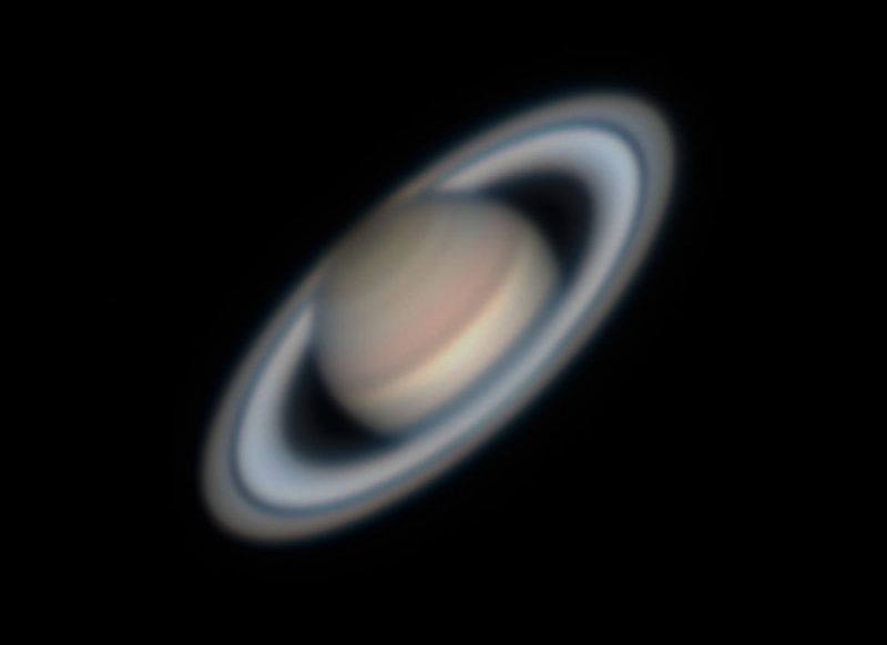
View at EarthSky Community Photos. | Patrick Prokop in Savannah, Georgia, caught this glorious image of golden Saturn on July 3, 2019. He wrote: “Saturn is at its best viewing for the year as it reaches opposition on July 9. That is the night that the Earth is between the sun and Saturn … Earth is about 93.2 million miles from the sun now while Saturn will be 841.4 million miles from us then. I took this picture shortly after midnight July 3 from my backyard. On July 9 it will be roughly a half million miles closer than it was at the time of this picture.” Thank you, Patrick!

There has been a lot of talk in recent weeks about exciting times for observing Jupiter and Saturn. That’s because both reach opposition in this northern summer of 2019, Jupiter on June 10 and Saturn on July 9. In fact, opposition happens yearly for both of these outer planets. It’s an event that marks the middle of the best time of year to view these planets. So … what is opposition?

Imagine the solar system, with the planets running around in their orbits. Let’s keep things simple and just imagine the sun in the middle with the Earth a little way out, Jupiter about five times farther, and then Saturn about twice as far away from the sun as Jupiter. We’ll assume we’re watching from a spot high above Earth’s North Pole, which would mean that everything is moving counterclockwise.

Now, hit pause. Where are the planets? Maybe Earth is off to the left of the sun, and maybe Jupiter and Saturn are to the right. From this view, it doesn’t really matter what the line from the sun to Earth is like; after all, there’s always a straight line between any two objects in space. But what’s the Earth-sun line doing with respect to, say, Saturn? For most of every year, the Earth-sun line would need to jog off in a different direction to get to Saturn.

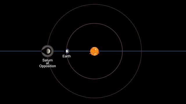
If we let our imaginary solar system run a little longer, though, the line will straighten. Nearly every year, there will be a point where it’s perfectly straight – sun, Earth, Saturn – as in the illustration below. Earth will be passing between Saturn and the sun in our planet’s yearly orbit.

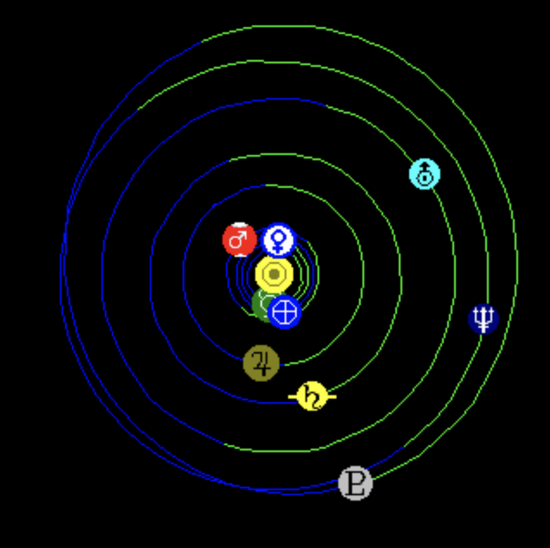
View larger. | An illustration of the solar system – as viewed from Earthly north – on the day of Saturn’s opposition. Earth is passing between Saturn and the sun. In this illustration, the yellow ball in the center (with the central dot) is the sun. Jupiter is brown; Saturn is yellow; Earth is blue. Everything is moving counterclockwise. Note that Earth passed between Jupiter at the sun last month, so that we are now racing ahead of this planet. Jupiter’s 2019 opposition was June 10. Earth passes between Saturn and the sun this week, on July 9. Diagram not to scale. Via Fourmilab.

What about the view in Earth’s sky? Since – at opposition – Earth is in the middle of a line between an outer planet and the sun, we see the sun at one end of our sky and the opposition planet in the opposite direction. It’s as if you’re standing directly between two friends as you chat in the supermarket, and you need to turn your head halfway around to see one, and then the other. At opposition, the sun is on the opposite side of the sky from the outer planet; when the sun sets in the west, the planet is rising in the east. As the planet drops below the horizon, the sun pops above it again – opposite.

To be technical, opposition for an outer planet happens when the sun and that planet are exactly 180 degrees apart in the sky. The word comes to English from a Latin root, meaning to set against.

Consider that Venus and Mercury can never be at opposition as seen from Earth. Their orbits are closer to the sun than Earth’s, so they can never appear opposite the sun in our sky. You will never see Venus in the east, for example, when the sun is setting in the west. These inner planets always stay near the sun, no more than 47 degrees from the sun for Venus, or 28 degrees for Mercury, in our sky.

Oppositions can only happen for objects that are father from the sun than Earth is. We see oppositions for Jupiter, Saturn, Uranus and Neptune about every year. They happen as Earth, in its much-faster orbit, passes between these outer worlds and the sun. We see oppositions of the planet Mars, too, but Martian oppositions happen about every 27 months because Earth and Mars are so relatively close together in orbit around the sun; their orbits, and speeds in orbit, are more similar. Since everything in space is always moving, oppositions of outer planets happen over and over, as Earth catches up and then passes the planet, on our inner track around the sun. As far as the bright planets go, the next opposition is never too far away:

Mars was at opposition on July 27, 2018, and will be again on October 13, 2020, and December 8, 2022.

Jupiter was at opposition on June 10, 2019, and will be again on July 14, 2020, August 19, 2021, and September 26, 2022.

Saturn will be at opposition on July 9, 2019, and then again on July 20, 2020, August 2, 2021, and August 14, 2022.

View full-sized image. | Project Nightflight released this photo on September 2, 2018. It shows Mars in mid-August, a couple of weeks after its late July opposition in 2018. See how bright it is? Planets at opposition are bright partly because it’s around then that they are closest to us. Also, at opposition, an outer planet’s fully lighted face, or day side, faces us most directly. Photo via the Project Nightflight team. Read more about this image.

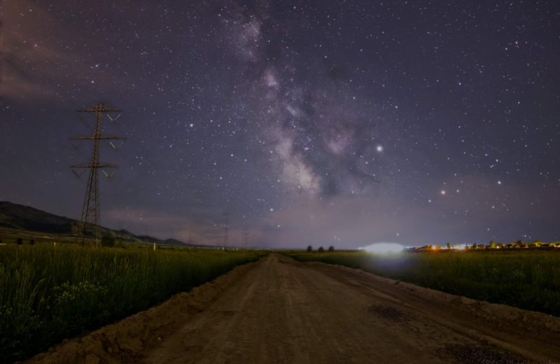
View at EarthSky Community Photos. | Eli Frisbie in Eagle Mountain, Utah, created this composite image from photos gathered on June 6, 2019, just a few days before Jupiter’s opposition. He wrote: “The Milky Way shines over a country road … The bright ‘star’ to the right of the Milky Way is the planet Jupiter. The slightly less-bright star to the upper left is the planet Saturn.” Thank you, Eli!

Why are planets at opposition so interesting to sky-watchers?

As mentioned, because they’re opposite the sun, planets at opposition rise when the sun sets and can be found somewhere in the sky throughout the night.

Secondly, planets at opposition tend to be near their closest point to Earth in orbit. Due to the non-circular shape of planetary orbits, the exact closest point might be different by a day or two, as Jupiter’s was this past June. Jupiter’s opposition was June 10, and its exact closest point was June 12. Still, for many weeks around opposition – between the time we pass between an outer planet and the sun – the outer planet is generally closest to Earth. At such a time, the planet is brightest, and more detail can be seen through telescopes.

And here’s another interesting aspect of opposition. Since the sun and outer planet are directly opposite each other in Earth’s sky, we see that far-off planet’s fully lighted daytime side. Fully-lit planets appear brighter to us than less-fully-lit planets. If you’re saying to yourself that this sounds a lot like the moon, you’re right! After all, what’s a full moon if not the moon at opposition? During the moon’s full phase, it’s directly opposite the sun in the sky, fully illuminated, and at its brightest for that orbit. As it moves through the rest of its orbit, the sun-Earth-moon line bends and gives us what we see from Earth as the moon’s phases.

Like so much in life, opposition is all about point of view. We’ve been talking about the view from Earth. What if we flip it around? When an outer planet – let’s say Jupiter – is at opposition for us, Earth is at inferior conjunction as seen from that planet. In other words, at the moment for us on Earth, observers on Jupiter would see Earth passing between their world and the sun. The Earth and the sun would be in the same side of Jupiter’s sky, hidden in the sun’s glare, except to skilled observers using special equipment. Consider also that the line from the sun to Jupiter passes through the Earth, which means Earth passes directly between the sun and Jupiter. Maybe one day, a visitor to Jupiter will see Earth transit the sun as seen from Jupiter. That is, they’ll see Earth’s darkened nighttime side, and all of humanity, cross the face of the sun from a half billion miles away.

Another artist’s concept of Saturn in opposition to the sun. Distances not to scale! Image via NASA.

Bottom Line: In astronomy, we say an outer planet is at opposition when it’s directly opposite the sun, rising at sunset. Opposition marks the middle of the best time of year to see an outer planet.

from EarthSky https://ift.tt/2L8UMSJ

View at EarthSky Community Photos. | Patrick Prokop in Savannah, Georgia, caught this glorious image of golden Saturn on July 3, 2019. He wrote: “Saturn is at its best viewing for the year as it reaches opposition on July 9. That is the night that the Earth is between the sun and Saturn … Earth is about 93.2 million miles from the sun now while Saturn will be 841.4 million miles from us then. I took this picture shortly after midnight July 3 from my backyard. On July 9 it will be roughly a half million miles closer than it was at the time of this picture.” Thank you, Patrick!

There has been a lot of talk in recent weeks about exciting times for observing Jupiter and Saturn. That’s because both reach opposition in this northern summer of 2019, Jupiter on June 10 and Saturn on July 9. In fact, opposition happens yearly for both of these outer planets. It’s an event that marks the middle of the best time of year to view these planets. So … what is opposition?

Imagine the solar system, with the planets running around in their orbits. Let’s keep things simple and just imagine the sun in the middle with the Earth a little way out, Jupiter about five times farther, and then Saturn about twice as far away from the sun as Jupiter. We’ll assume we’re watching from a spot high above Earth’s North Pole, which would mean that everything is moving counterclockwise.

Now, hit pause. Where are the planets? Maybe Earth is off to the left of the sun, and maybe Jupiter and Saturn are to the right. From this view, it doesn’t really matter what the line from the sun to Earth is like; after all, there’s always a straight line between any two objects in space. But what’s the Earth-sun line doing with respect to, say, Saturn? For most of every year, the Earth-sun line would need to jog off in a different direction to get to Saturn.

If we let our imaginary solar system run a little longer, though, the line will straighten. Nearly every year, there will be a point where it’s perfectly straight – sun, Earth, Saturn – as in the illustration below. Earth will be passing between Saturn and the sun in our planet’s yearly orbit.

View larger. | An illustration of the solar system – as viewed from Earthly north – on the day of Saturn’s opposition. Earth is passing between Saturn and the sun. In this illustration, the yellow ball in the center (with the central dot) is the sun. Jupiter is brown; Saturn is yellow; Earth is blue. Everything is moving counterclockwise. Note that Earth passed between Jupiter at the sun last month, so that we are now racing ahead of this planet. Jupiter’s 2019 opposition was June 10. Earth passes between Saturn and the sun this week, on July 9. Diagram not to scale. Via Fourmilab.

What about the view in Earth’s sky? Since – at opposition – Earth is in the middle of a line between an outer planet and the sun, we see the sun at one end of our sky and the opposition planet in the opposite direction. It’s as if you’re standing directly between two friends as you chat in the supermarket, and you need to turn your head halfway around to see one, and then the other. At opposition, the sun is on the opposite side of the sky from the outer planet; when the sun sets in the west, the planet is rising in the east. As the planet drops below the horizon, the sun pops above it again – opposite.

To be technical, opposition for an outer planet happens when the sun and that planet are exactly 180 degrees apart in the sky. The word comes to English from a Latin root, meaning to set against.

Consider that Venus and Mercury can never be at opposition as seen from Earth. Their orbits are closer to the sun than Earth’s, so they can never appear opposite the sun in our sky. You will never see Venus in the east, for example, when the sun is setting in the west. These inner planets always stay near the sun, no more than 47 degrees from the sun for Venus, or 28 degrees for Mercury, in our sky.

Oppositions can only happen for objects that are father from the sun than Earth is. We see oppositions for Jupiter, Saturn, Uranus and Neptune about every year. They happen as Earth, in its much-faster orbit, passes between these outer worlds and the sun. We see oppositions of the planet Mars, too, but Martian oppositions happen about every 27 months because Earth and Mars are so relatively close together in orbit around the sun; their orbits, and speeds in orbit, are more similar. Since everything in space is always moving, oppositions of outer planets happen over and over, as Earth catches up and then passes the planet, on our inner track around the sun. As far as the bright planets go, the next opposition is never too far away:

Mars was at opposition on July 27, 2018, and will be again on October 13, 2020, and December 8, 2022.

Jupiter was at opposition on June 10, 2019, and will be again on July 14, 2020, August 19, 2021, and September 26, 2022.

Saturn will be at opposition on July 9, 2019, and then again on July 20, 2020, August 2, 2021, and August 14, 2022.

View full-sized image. | Project Nightflight released this photo on September 2, 2018. It shows Mars in mid-August, a couple of weeks after its late July opposition in 2018. See how bright it is? Planets at opposition are bright partly because it’s around then that they are closest to us. Also, at opposition, an outer planet’s fully lighted face, or day side, faces us most directly. Photo via the Project Nightflight team. Read more about this image.

View at EarthSky Community Photos. | Eli Frisbie in Eagle Mountain, Utah, created this composite image from photos gathered on June 6, 2019, just a few days before Jupiter’s opposition. He wrote: “The Milky Way shines over a country road … The bright ‘star’ to the right of the Milky Way is the planet Jupiter. The slightly less-bright star to the upper left is the planet Saturn.” Thank you, Eli!

Why are planets at opposition so interesting to sky-watchers?

As mentioned, because they’re opposite the sun, planets at opposition rise when the sun sets and can be found somewhere in the sky throughout the night.

Secondly, planets at opposition tend to be near their closest point to Earth in orbit. Due to the non-circular shape of planetary orbits, the exact closest point might be different by a day or two, as Jupiter’s was this past June. Jupiter’s opposition was June 10, and its exact closest point was June 12. Still, for many weeks around opposition – between the time we pass between an outer planet and the sun – the outer planet is generally closest to Earth. At such a time, the planet is brightest, and more detail can be seen through telescopes.

And here’s another interesting aspect of opposition. Since the sun and outer planet are directly opposite each other in Earth’s sky, we see that far-off planet’s fully lighted daytime side. Fully-lit planets appear brighter to us than less-fully-lit planets. If you’re saying to yourself that this sounds a lot like the moon, you’re right! After all, what’s a full moon if not the moon at opposition? During the moon’s full phase, it’s directly opposite the sun in the sky, fully illuminated, and at its brightest for that orbit. As it moves through the rest of its orbit, the sun-Earth-moon line bends and gives us what we see from Earth as the moon’s phases.

Like so much in life, opposition is all about point of view. We’ve been talking about the view from Earth. What if we flip it around? When an outer planet – let’s say Jupiter – is at opposition for us, Earth is at inferior conjunction as seen from that planet. In other words, at the moment for us on Earth, observers on Jupiter would see Earth passing between their world and the sun. The Earth and the sun would be in the same side of Jupiter’s sky, hidden in the sun’s glare, except to skilled observers using special equipment. Consider also that the line from the sun to Jupiter passes through the Earth, which means Earth passes directly between the sun and Jupiter. Maybe one day, a visitor to Jupiter will see Earth transit the sun as seen from Jupiter. That is, they’ll see Earth’s darkened nighttime side, and all of humanity, cross the face of the sun from a half billion miles away.

Another artist’s concept of Saturn in opposition to the sun. Distances not to scale! Image via NASA.

Bottom Line: In astronomy, we say an outer planet is at opposition when it’s directly opposite the sun, rising at sunset. Opposition marks the middle of the best time of year to see an outer planet.

from EarthSky https://ift.tt/2L8UMSJ

Today in 2003: Opportunity blasts off to Mars

The dramatic image of NASA’s Mars Exploration Rover Opportunity’s shadow was taken on sol 180 (July 26, 2004) by the rover’s front hazard-avoidance camera as the rover moved farther into Endurance Crater in the Meridiani Planum region of Mars. Image via NASA/JPL-Caltech.

July 7, 2003. On this date, NASA’s Mars rover Opportunity blasted off on a journey to Mars. After traveling for some seven months through space, Opportunity landed on Mars’ Meridiani Planum on January 25, 2004, three weeks after its twin rover Spirit touched down on the other side of the planet. Spirit stopped moving across Mars’ surface in 2009, and it stopped sending back signals to Earth in 2010. Meanwhile, Opportunity – designed to last just 90 Martian days and travel 1,100 yards (1,000 meters) across Mars’ surface – vastly surpassed all expectations in its endurance, scientific value and longevity. It became one of the most successful feats of interplanetary exploration, effectively ending in 2018 (and officially ending in 2019) after some 15 years exploring the surface of Mars.

In addition to exceeding its life expectancy by 60 times, the rover traveled more than 28 miles (45 km) by the time it reached its most appropriate final resting spot in Mars’ Perseverance Valley. The Opportunity rover stopped communicating with Earth when a severe Mars-wide dust storm blanketed its location in June 2018. Presumably, the storm affected the rover’s solar panels. Opportunity’s final communication was received June 10, 2018.

A layer of dust covers Opportunity’s solar arrays following a dust storm in January 2014, left, but by March 2014 much of the dust had blown away. Image via NASA/JPL Caltech/Cornell/Arizona State.

But NASA didn’t know that yet. Throughout the late summer and fall of 2018, engineers in the Space Flight Operations Facility at NASA’s Jet Propulsion Laboratory (JPL) conducted a multifaceted, eight-month recovery strategy in an attempt to compel the rover to communicate. They sent more than a thousand commands to the rover … but there was no response. In what became a months-long outpouring of emotion, space fans on Twitter and other social media platforms began using the hashtags #ThankYouOppy and #GoodnightOppy.

Space engineers made their last attempt to revive Opportunity on February 12, 2019, starting with a “wake-up song” played in the control room at JPL. The mission’s principal investigator, Steve Squyres, had chosen I’ll Be Seeing You, as performed by Billie Holiday. At 8:10 p.m., Holiday’s wistful voice floated up from the command floor:

I’ll be seeing you in all the old familiar places that this heart of mine embraces.

As was expected by that time, those final efforts at communication were to no avail. Opportunity remained silent on the surface of Mars. Project manager John Callas told the crowd of NASA employees gathered for the farewell transmission:

This is a hard day. Even though it’s a machine and we’re saying goodbye, it’s still very hard and very poignant, but we had to do that. We came to that point.

Artist’s concept of the Mars Opportunity rover. Image via NASA.

From the day Opportunity landed, a team of mission engineers, rover drivers and scientists on Earth collaborated to overcome challenges and get the rover from one geologic site on Mars to the next. They plotted workable avenues over rugged terrain so that the 384-pound (174-kilogram) Martian explorer could maneuver around and, at times, over rocks and boulders, climb gravel-strewn slopes as steep as 32 degrees (an off-Earth record), probe crater floors, summit hills and traverse possible dry riverbeds. Its final venture brought it to the western limb of Perseverance Valley. Opportunity’s achievements include:

– Setting a one-day Mars driving record March 20, 2005, when it traveled 721 feet (220 meters).
– Returning more than 217,000 images, including 15 360-degree color panoramas.
– Exposing the surfaces of 52 rocks to reveal fresh mineral surfaces for analysis and cleared 72 additional targets with a brush to prepare them for inspection with spectrometers and a microscopic imager.
– Finding hematite, a mineral that forms in water, at its landing site.
– Discovering strong indications at Endeavour Crater of the action of ancient water similar to the drinkable water of a pond or lake on Earth.

In the video below, Steve Squyres speaks about Opportunity’s mission and its significance

All those accomplishments were not without the occasional extraterrestrial impediment. In 2005 alone, Opportunity lost steering to one of its front wheels, a stuck heater threatened to severely limit the rover’s available power, and a Martian sand ripple almost trapped it for good. Two years later, a two-month dust storm imperiled the rover before relenting. In 2015, Opportunity lost use of its 256-megabyte flash memory and, in 2017, it lost steering to its other front wheel.

Each time the rover faced an obstacle, Opportunity’s team on Earth found and implemented a solution that enabled the rover to bounce back. However, the massive dust storm that took shape in the summer of 2018 proved too much for history’s most senior Mars explorer.

Mars exploration continues. NASA’s InSight lander, which touched down on November 26, 2018, is just beginning its scientific investigations. The Curiosity rover has been exploring Gale Crater for more than six years. And, NASA’s Mars 2020 rover and the European Space Agency’s ExoMars rover both will launch in July 2020, becoming the first rover missions designed to seek signs of past microbial life on the red planet.

The Opportunity rover featured an array of scientific tools. One of its main objectives was the search for signs of water on the red planet, since, as far as we know, water is necessary for life. Image via NASA/JPL-Caltech/Cornell.

Bottom line: NASA’s Opportunity rover launched to Mars on July 7, 2003. It officially ended its mission on February 13, 2019.

from EarthSky https://ift.tt/32hb5ST

The dramatic image of NASA’s Mars Exploration Rover Opportunity’s shadow was taken on sol 180 (July 26, 2004) by the rover’s front hazard-avoidance camera as the rover moved farther into Endurance Crater in the Meridiani Planum region of Mars. Image via NASA/JPL-Caltech.

July 7, 2003. On this date, NASA’s Mars rover Opportunity blasted off on a journey to Mars. After traveling for some seven months through space, Opportunity landed on Mars’ Meridiani Planum on January 25, 2004, three weeks after its twin rover Spirit touched down on the other side of the planet. Spirit stopped moving across Mars’ surface in 2009, and it stopped sending back signals to Earth in 2010. Meanwhile, Opportunity – designed to last just 90 Martian days and travel 1,100 yards (1,000 meters) across Mars’ surface – vastly surpassed all expectations in its endurance, scientific value and longevity. It became one of the most successful feats of interplanetary exploration, effectively ending in 2018 (and officially ending in 2019) after some 15 years exploring the surface of Mars.

In addition to exceeding its life expectancy by 60 times, the rover traveled more than 28 miles (45 km) by the time it reached its most appropriate final resting spot in Mars’ Perseverance Valley. The Opportunity rover stopped communicating with Earth when a severe Mars-wide dust storm blanketed its location in June 2018. Presumably, the storm affected the rover’s solar panels. Opportunity’s final communication was received June 10, 2018.

A layer of dust covers Opportunity’s solar arrays following a dust storm in January 2014, left, but by March 2014 much of the dust had blown away. Image via NASA/JPL Caltech/Cornell/Arizona State.

But NASA didn’t know that yet. Throughout the late summer and fall of 2018, engineers in the Space Flight Operations Facility at NASA’s Jet Propulsion Laboratory (JPL) conducted a multifaceted, eight-month recovery strategy in an attempt to compel the rover to communicate. They sent more than a thousand commands to the rover … but there was no response. In what became a months-long outpouring of emotion, space fans on Twitter and other social media platforms began using the hashtags #ThankYouOppy and #GoodnightOppy.

Space engineers made their last attempt to revive Opportunity on February 12, 2019, starting with a “wake-up song” played in the control room at JPL. The mission’s principal investigator, Steve Squyres, had chosen I’ll Be Seeing You, as performed by Billie Holiday. At 8:10 p.m., Holiday’s wistful voice floated up from the command floor:

I’ll be seeing you in all the old familiar places that this heart of mine embraces.

As was expected by that time, those final efforts at communication were to no avail. Opportunity remained silent on the surface of Mars. Project manager John Callas told the crowd of NASA employees gathered for the farewell transmission:

This is a hard day. Even though it’s a machine and we’re saying goodbye, it’s still very hard and very poignant, but we had to do that. We came to that point.

Artist’s concept of the Mars Opportunity rover. Image via NASA.

From the day Opportunity landed, a team of mission engineers, rover drivers and scientists on Earth collaborated to overcome challenges and get the rover from one geologic site on Mars to the next. They plotted workable avenues over rugged terrain so that the 384-pound (174-kilogram) Martian explorer could maneuver around and, at times, over rocks and boulders, climb gravel-strewn slopes as steep as 32 degrees (an off-Earth record), probe crater floors, summit hills and traverse possible dry riverbeds. Its final venture brought it to the western limb of Perseverance Valley. Opportunity’s achievements include:

– Setting a one-day Mars driving record March 20, 2005, when it traveled 721 feet (220 meters).
– Returning more than 217,000 images, including 15 360-degree color panoramas.
– Exposing the surfaces of 52 rocks to reveal fresh mineral surfaces for analysis and cleared 72 additional targets with a brush to prepare them for inspection with spectrometers and a microscopic imager.
– Finding hematite, a mineral that forms in water, at its landing site.
– Discovering strong indications at Endeavour Crater of the action of ancient water similar to the drinkable water of a pond or lake on Earth.

In the video below, Steve Squyres speaks about Opportunity’s mission and its significance

All those accomplishments were not without the occasional extraterrestrial impediment. In 2005 alone, Opportunity lost steering to one of its front wheels, a stuck heater threatened to severely limit the rover’s available power, and a Martian sand ripple almost trapped it for good. Two years later, a two-month dust storm imperiled the rover before relenting. In 2015, Opportunity lost use of its 256-megabyte flash memory and, in 2017, it lost steering to its other front wheel.

Each time the rover faced an obstacle, Opportunity’s team on Earth found and implemented a solution that enabled the rover to bounce back. However, the massive dust storm that took shape in the summer of 2018 proved too much for history’s most senior Mars explorer.

Mars exploration continues. NASA’s InSight lander, which touched down on November 26, 2018, is just beginning its scientific investigations. The Curiosity rover has been exploring Gale Crater for more than six years. And, NASA’s Mars 2020 rover and the European Space Agency’s ExoMars rover both will launch in July 2020, becoming the first rover missions designed to seek signs of past microbial life on the red planet.

The Opportunity rover featured an array of scientific tools. One of its main objectives was the search for signs of water on the red planet, since, as far as we know, water is necessary for life. Image via NASA/JPL-Caltech/Cornell.

Bottom line: NASA’s Opportunity rover launched to Mars on July 7, 2003. It officially ended its mission on February 13, 2019.

from EarthSky https://ift.tt/32hb5ST

Use Big Dipper to find Polaris

Tonight, use the Big Dipper in the constellation Ursa Major the Great Bear to find the sky’s northern pole star, Polaris. This is the star around which the whole northern celestial sphere appears to turn throughout the night. That’s because this star is located nearly above Earth’s northern axis. In times past, wanderers on the northern face of Earth used Polaris to stay on course.

Once you find it, you can also look for Thuban, a famous former pole star in the constellation Draco the Dragon. More about finding Thuban below.

So how can you find Polaris? Look at the chart at the top of this post. You’ll simply draw a line through the Big Dipper’s pointer stars – Dubhe and Merak. That line will point to Polaris, the North Star. You can use this trick to find Polaris any evening – no matter how the Dipper is oriented with respect to your northern horizon.

EarthSky community member Ken Christison captured these glorious star trails around Polaris, the North Star. This is the star around which the entire northern sky appears to turn.

Once you’ve got Polaris, if your sky is dark enough, you might be able to see the Little Dipper asterism. It’s harder to spot than the Big Dipper and needs a dark sky to be seen.

The chart below shows the Big Dipper, Little Dipper and the star Polaris as you’ll see them in the north on July evenings. Polaris marks the end of the handle on the Little Dipper asterism, which is in the constellation Ursa Minor.

In other words, the Little Dipper is not the whole constellation, but just a noticeable pattern within the constellation Ursa Minor the Smaller Bear.

Polaris isn’t the brightest star in the sky, as is commonly supposed. It’s only 50th brightest or so.

Still, Polaris is bright enough to be seen with relative ease on a dark, clear night.

Enjoying EarthSky so far? Sign up for our free daily newsletter today!

Orientation of Dippers on July evenings. Note that Polaris is the end star in the handle of the Little Dipper. And look at Thuban, between the Dippers.

How to find the star Thuban, and its constellation Draco the Dragon. As night deepens, and the fainter stars of the Little Dipper spring into view, those of you with dark-enough skies can expect to see a winding stream of stars between the Big and Little Dippers. These meandering stars make up the constellation Draco.

The star Thuban is one of the stars here, part of the Tail of the legendary constellation Draco the Dragon, a fixture of the northern skies. I always find Thuban by remembering it’s between the Big and Little Dippers.

Thuban is famous for having served as a pole star around 3000 B.C. This date coincides with the beginning of the building of the pyramids in Egypt. It’s said that the descending passage of the Great Pyramid of Khufu at Gizeh was built to point directly at Thuban. So our ancestors knew and celebrated this star.

More about Draco, the great Dragon of the north

Draco the Dragon as seen on early summer evenings from mid-northern latitudes. Image via AlltheSky.com

Bottom line: Draw a line through the Big Dipper pointer stars to find Polaris the North Star. If your sky is dark, look for Thuban in the Tail of Draco the Dragon.

July 2019 guide to the bright planets

Donate: Your support means the world to us

from EarthSky https://ift.tt/2Jgnlv8

Tonight, use the Big Dipper in the constellation Ursa Major the Great Bear to find the sky’s northern pole star, Polaris. This is the star around which the whole northern celestial sphere appears to turn throughout the night. That’s because this star is located nearly above Earth’s northern axis. In times past, wanderers on the northern face of Earth used Polaris to stay on course.

Once you find it, you can also look for Thuban, a famous former pole star in the constellation Draco the Dragon. More about finding Thuban below.

So how can you find Polaris? Look at the chart at the top of this post. You’ll simply draw a line through the Big Dipper’s pointer stars – Dubhe and Merak. That line will point to Polaris, the North Star. You can use this trick to find Polaris any evening – no matter how the Dipper is oriented with respect to your northern horizon.

EarthSky community member Ken Christison captured these glorious star trails around Polaris, the North Star. This is the star around which the entire northern sky appears to turn.

Once you’ve got Polaris, if your sky is dark enough, you might be able to see the Little Dipper asterism. It’s harder to spot than the Big Dipper and needs a dark sky to be seen.

The chart below shows the Big Dipper, Little Dipper and the star Polaris as you’ll see them in the north on July evenings. Polaris marks the end of the handle on the Little Dipper asterism, which is in the constellation Ursa Minor.

In other words, the Little Dipper is not the whole constellation, but just a noticeable pattern within the constellation Ursa Minor the Smaller Bear.

Polaris isn’t the brightest star in the sky, as is commonly supposed. It’s only 50th brightest or so.

Still, Polaris is bright enough to be seen with relative ease on a dark, clear night.

Enjoying EarthSky so far? Sign up for our free daily newsletter today!

Orientation of Dippers on July evenings. Note that Polaris is the end star in the handle of the Little Dipper. And look at Thuban, between the Dippers.

How to find the star Thuban, and its constellation Draco the Dragon. As night deepens, and the fainter stars of the Little Dipper spring into view, those of you with dark-enough skies can expect to see a winding stream of stars between the Big and Little Dippers. These meandering stars make up the constellation Draco.

The star Thuban is one of the stars here, part of the Tail of the legendary constellation Draco the Dragon, a fixture of the northern skies. I always find Thuban by remembering it’s between the Big and Little Dippers.

Thuban is famous for having served as a pole star around 3000 B.C. This date coincides with the beginning of the building of the pyramids in Egypt. It’s said that the descending passage of the Great Pyramid of Khufu at Gizeh was built to point directly at Thuban. So our ancestors knew and celebrated this star.

More about Draco, the great Dragon of the north

Draco the Dragon as seen on early summer evenings from mid-northern latitudes. Image via AlltheSky.com

Bottom line: Draw a line through the Big Dipper pointer stars to find Polaris the North Star. If your sky is dark, look for Thuban in the Tail of Draco the Dragon.

July 2019 guide to the bright planets

Donate: Your support means the world to us

from EarthSky https://ift.tt/2Jgnlv8

2019 SkS Weekly Climate Change & Global Warming News Roundup #27

A chronological listing of news articles posted on the Skeptical Science Facebook Page during the past week, i.e., Sun, Jun 30 through Sat, July 6, 2019

Editor's Pick

German environment minister proposes carbon tax

Svenja Schulze has said such a plan is important for sinking carbon emissions, yet other measures are needed. She claims the plan would not unduly burden the poor, but reward those who use less fuel.

 

Germany's Social Democrat (SPD) Environment Minister Svenja Schulze presented three independent studies on possible carbon tax schemes in Berlin on Friday. Insisting such a tax would not unduly burden the poor, she said, "those who decide to live a more climate-friendly life could actually get money back."

The plans Schulze presented suggested an initial €35 ($39.50) tax on each metric ton of CO2, to be increased to €180 by 2030. The idea being that the more expensive petrol, natural gas, and heating oil become, the less people will use.

Schulze told reporters that those who consume less, including children, will be given a so-called climate bonus of up to €100 per person, per year, which she claims would offset a person's outlay for the tax, "The less you drive, the less oil you burn, the more you will get back."

The minister underscored the importance of not burdening low and middle-class families: "It's really important to me to avoid unfairly burdening those with low and medium incomes, and especially affected groups like commuters and tenants." 

German environment minister proposes carbon tax, Deutsche Welle (DW), July 5, 2019 

---

Links posted on Facebook

Sun June 30, 2019

• How Republican senators killed Oregon’s climate crisis bill by Jason Wilson, US News, Guardian, June 29, 2019
• Protective Wind Shear Barrier Against Hurricanes on Southeast U.S. Coast Likely to Weaken in Coming Decades by Jeff Masters, Category 6, Weather Underground, June 24, 2019
• "I'm Not Willing to Do That": Trump Says He Won't Take Climate Action Because It Would Threaten Corporate Profits by Jake Johnson, Common Dreams, June 29, 2019
• United States remains outlier as G20 split over tackling climate change by Malcolm Foster & Chang-Ran Kim, Reuters, June 29, 2019
• Is climate change an “existential threat” — or just a catastrophic one? by Kelsey Piper, Future Perfect, Vox, June 28, 2019
• Religion must rise to the challenge of climate change too, Opinion by Graham Lawton, Environment, New Scientists, June 19, 2019
• If Climate Change Doesn't Kill Me, My Anxiety About It Will by Véronique Hyland Elle Magazine, June 9, 2019
• 4 Reasons Climate Change Impacts On Agriculture Matter To You by Marshall Shepherd, Science, Forbes, June 26, 2019

Mon July 1, 2019

• Heatwave cooks mussels in their shells on California shore by Susie Cagle, Environment, Guardian, June 29, 2019
• GE’s Multi-Billion Dollar Mistake by Molly Taft, Nexus Media News, June 26, 2019
• Flood apocalypse in Eastern Siberia kills five and maroons 9,919 whose homes destroyed or damaged, The Siberian Times, June 30, 3019
• Europe’s record heat wave is changing stubborn minds about the value of air conditioning by Rick Noack, World, Washington Post, June 28, 2019
• No End in Sight for Record Midwest Flood Crisis by Daniel Cusick, E&E News/Scientific American, June 26, 2019
• We have too many fossil-fuel power plants to meet climate goals by Stephen Leahy, Environment, National Geographic, July 1, 2019
• Precipitous' fall in Antarctic sea ice since 2014 revealed by Damian Carrington, Environment, Guardian, July 1, 2019
• The problem with predicting the end the world by Matthew Rozsa, Salon, June 30, 2019

Tue July 2, 2019

• Europe dodged a Bullet during Record June Heatwave, Climate State, July 1, 2019
• Chubb cuts coal insurance exposure because of climate change, Business, BBC News, July 1, 2019
• Nuclear Power, Once Seen as Impervious to Climate Change, Threatened by Heat Waves by Alan Neuhauser, National, US News & World Report, July 1, 2019
• France’s record-breaking heatwave made ‘at least five times’ more likely by climate change by Daisy Dunne, Carbon Brief, July 2, 2019
• Revealed: rampant deforestation of Amazon driven by global greed for meat by Dom Phillips, Daniel Camargos, Andre Campos, Andrew Wasley & Alexandra Heal, Environment, Guardian, July 2, 2019
• Planned growth of UK airports not consistent with net-zero climate goal, Guest Post by Declan Finney & Giulio Mattioli, Carbon Brief, June 24, 2019
• Donald Trump USDA Climate Science Quash Squanders US Science Leadership, YouTube Video by Rachel Maddow Show, MSNBC, June 1, 2019
• U.S. Mayors Pressure Congress on Carbon Pricing, Climate Lawsuits and a Green New Deal by Marianne Lavelle, InsideClimate News, July 1, 2019

Wed July 3, 2019

• Cities are beginning to own up to the climate impacts of what they consume by David Roberts, Energy & Environment, Vox, July 1, 2019
• Baked Alaska: record heat fuels wildfires and sends tourists to the beach by Susie Cagle, Environment, Guardian, July 3, 2019
• Bonn climate talks: Key outcomes from the June 2019 UN climate conference by Josh Gabbatiss, Carbon Brief, July 1, 2019
• It takes years to fully recover from big storms like Sandy by Jack L Harris, The Conversation US, July 2, 2019
• Meet generation Greta: young climate activists around the world by Anna Turns, Environment, Guardian, June 28, 2019
• Exclusive: Investors with $34 trillion demand urgent climate change action by Simon Jessop & Nina Chestney, Sustainable Business,  Reuters, June 25, 2019
• Europe's Extreme Heat Wave Had Climate Change Fingerprints, Study Says by Bob Berwyn, InsideClimate News, July 3, 2019
• Welcome to the fastest-heating place on Earth place on Earth by Jonathan Watts, Environment (Interactive), Guardian, July 1, 2019

Thur July 4, 2019

• An Ancient City’s Demise Hints at a Hidden Risk of Sea-Level Rise by Parker Richards, Science, The Atlantic Magazine, June 28, 2019
• We must not barter the Amazon rainforest for burgers and steaks, Opinion by Jonathan Watts, Comment is Free, Guardian, July 2, 2019
• A giant heat dome over Alaska is set to threaten all-time temperature records by Ian Livingston, Capital Weather Gang, Washington Post, July 3, 2019
• Are parts of India becoming too hot for humans? by Shekhar Chandra, CNN, July 3, 2019
• 8 Essential Steps to Radically Transform Our Economy, Opinion by David Korten, New Economy, YES! Magazine, July 2, 2019
• Keep climate teaching real and honest by Anne Kagoya, Climate News Network, July 4, 2019
• Governments and firms in 28 countries sued over climate crisis – report by Sandra Laville, Environment, Guardian, July 4, 2019
• Do Americans Need Air-Conditioning? by Penelope Green, Style, New York Times, July 3, 2019

Fri July 5, 2019

• We must face climate emergency head-on by Quentin Atkinson, ideasroom, newsroom.co.nz, July 4, 2018
• Climate campaigners 'greatest threat' to oil sector: OPEC, AFP, July 2, 2019
• India staring at a water apocalypse by Saikat Datta, India, Asia Times, July 2, 2019
• 10 things a committed U.S. President and Congress could do about climate change, Commentary by Craig K. Chandler, Yale Climate Connections, June 25, 2019
• Redefining hope in a world threatened by climate change by SueEllen Campbell, Yale Climate Connections, July 5, 2019
• Climate change: Trees 'most effective solution' for warming by Matt McGrath, Science & Environment, BBC News, July 4, 2019
• 'Revolutionise the world’: UN chief calls for youth to lead on Jclimate by Chloé Farand, Climate Home News, June 30, 2019
• ‘Our biggest compliment yet’: Greta Thunberg thanks OPEC for criticism by Sam Meredith, CNBC News, Jul 5, 2019

Sat July 6, 2019

• UK Government Agency's Annual Support for Overseas Fossil Fuel Projects Rises to £2bn by Simon Roach & Richard Collett-White, DeSmog UK, June 27, 2019
• Booming LNG industry could be as bad for climate as coal, experts warn by Adam Morton, Environment, Guardian, July 2, 2019
• The Powerpoint That Got a Climate Scientist Disinvited from a Shell Conference by Kate Aronoff, The Intercept, July 5, 2019
• Electric cars 'will not solve transport problem,' report warns by Roger Harrabin, BBC News, July 5, 2019
• A ‘Climate Emergency’ Was Declared in New York City. Will That Change Anything? by Anne Barnard, New York Times, July 5, 2019
• German environment minister proposes carbon tax, Deutsche Welle (DW), July 5, 2019

from Skeptical Science https://ift.tt/2FX9I21

A chronological listing of news articles posted on the Skeptical Science Facebook Page during the past week, i.e., Sun, Jun 30 through Sat, July 6, 2019

Editor's Pick

German environment minister proposes carbon tax

Svenja Schulze has said such a plan is important for sinking carbon emissions, yet other measures are needed. She claims the plan would not unduly burden the poor, but reward those who use less fuel.

 

Germany's Social Democrat (SPD) Environment Minister Svenja Schulze presented three independent studies on possible carbon tax schemes in Berlin on Friday. Insisting such a tax would not unduly burden the poor, she said, "those who decide to live a more climate-friendly life could actually get money back."

The plans Schulze presented suggested an initial €35 ($39.50) tax on each metric ton of CO2, to be increased to €180 by 2030. The idea being that the more expensive petrol, natural gas, and heating oil become, the less people will use.

Schulze told reporters that those who consume less, including children, will be given a so-called climate bonus of up to €100 per person, per year, which she claims would offset a person's outlay for the tax, "The less you drive, the less oil you burn, the more you will get back."

The minister underscored the importance of not burdening low and middle-class families: "It's really important to me to avoid unfairly burdening those with low and medium incomes, and especially affected groups like commuters and tenants." 

German environment minister proposes carbon tax, Deutsche Welle (DW), July 5, 2019 

---

Links posted on Facebook

Sun June 30, 2019

• How Republican senators killed Oregon’s climate crisis bill by Jason Wilson, US News, Guardian, June 29, 2019
• Protective Wind Shear Barrier Against Hurricanes on Southeast U.S. Coast Likely to Weaken in Coming Decades by Jeff Masters, Category 6, Weather Underground, June 24, 2019
• "I'm Not Willing to Do That": Trump Says He Won't Take Climate Action Because It Would Threaten Corporate Profits by Jake Johnson, Common Dreams, June 29, 2019
• United States remains outlier as G20 split over tackling climate change by Malcolm Foster & Chang-Ran Kim, Reuters, June 29, 2019
• Is climate change an “existential threat” — or just a catastrophic one? by Kelsey Piper, Future Perfect, Vox, June 28, 2019
• Religion must rise to the challenge of climate change too, Opinion by Graham Lawton, Environment, New Scientists, June 19, 2019
• If Climate Change Doesn't Kill Me, My Anxiety About It Will by Véronique Hyland Elle Magazine, June 9, 2019
• 4 Reasons Climate Change Impacts On Agriculture Matter To You by Marshall Shepherd, Science, Forbes, June 26, 2019

Mon July 1, 2019

• Heatwave cooks mussels in their shells on California shore by Susie Cagle, Environment, Guardian, June 29, 2019
• GE’s Multi-Billion Dollar Mistake by Molly Taft, Nexus Media News, June 26, 2019
• Flood apocalypse in Eastern Siberia kills five and maroons 9,919 whose homes destroyed or damaged, The Siberian Times, June 30, 3019
• Europe’s record heat wave is changing stubborn minds about the value of air conditioning by Rick Noack, World, Washington Post, June 28, 2019
• No End in Sight for Record Midwest Flood Crisis by Daniel Cusick, E&E News/Scientific American, June 26, 2019
• We have too many fossil-fuel power plants to meet climate goals by Stephen Leahy, Environment, National Geographic, July 1, 2019
• Precipitous' fall in Antarctic sea ice since 2014 revealed by Damian Carrington, Environment, Guardian, July 1, 2019
• The problem with predicting the end the world by Matthew Rozsa, Salon, June 30, 2019

Tue July 2, 2019

• Europe dodged a Bullet during Record June Heatwave, Climate State, July 1, 2019
• Chubb cuts coal insurance exposure because of climate change, Business, BBC News, July 1, 2019
• Nuclear Power, Once Seen as Impervious to Climate Change, Threatened by Heat Waves by Alan Neuhauser, National, US News & World Report, July 1, 2019
• France’s record-breaking heatwave made ‘at least five times’ more likely by climate change by Daisy Dunne, Carbon Brief, July 2, 2019
• Revealed: rampant deforestation of Amazon driven by global greed for meat by Dom Phillips, Daniel Camargos, Andre Campos, Andrew Wasley & Alexandra Heal, Environment, Guardian, July 2, 2019
• Planned growth of UK airports not consistent with net-zero climate goal, Guest Post by Declan Finney & Giulio Mattioli, Carbon Brief, June 24, 2019
• Donald Trump USDA Climate Science Quash Squanders US Science Leadership, YouTube Video by Rachel Maddow Show, MSNBC, June 1, 2019
• U.S. Mayors Pressure Congress on Carbon Pricing, Climate Lawsuits and a Green New Deal by Marianne Lavelle, InsideClimate News, July 1, 2019

Wed July 3, 2019

• Cities are beginning to own up to the climate impacts of what they consume by David Roberts, Energy & Environment, Vox, July 1, 2019
• Baked Alaska: record heat fuels wildfires and sends tourists to the beach by Susie Cagle, Environment, Guardian, July 3, 2019
• Bonn climate talks: Key outcomes from the June 2019 UN climate conference by Josh Gabbatiss, Carbon Brief, July 1, 2019
• It takes years to fully recover from big storms like Sandy by Jack L Harris, The Conversation US, July 2, 2019
• Meet generation Greta: young climate activists around the world by Anna Turns, Environment, Guardian, June 28, 2019
• Exclusive: Investors with $34 trillion demand urgent climate change action by Simon Jessop & Nina Chestney, Sustainable Business,  Reuters, June 25, 2019
• Europe's Extreme Heat Wave Had Climate Change Fingerprints, Study Says by Bob Berwyn, InsideClimate News, July 3, 2019
• Welcome to the fastest-heating place on Earth place on Earth by Jonathan Watts, Environment (Interactive), Guardian, July 1, 2019

Thur July 4, 2019

• An Ancient City’s Demise Hints at a Hidden Risk of Sea-Level Rise by Parker Richards, Science, The Atlantic Magazine, June 28, 2019
• We must not barter the Amazon rainforest for burgers and steaks, Opinion by Jonathan Watts, Comment is Free, Guardian, July 2, 2019
• A giant heat dome over Alaska is set to threaten all-time temperature records by Ian Livingston, Capital Weather Gang, Washington Post, July 3, 2019
• Are parts of India becoming too hot for humans? by Shekhar Chandra, CNN, July 3, 2019
• 8 Essential Steps to Radically Transform Our Economy, Opinion by David Korten, New Economy, YES! Magazine, July 2, 2019
• Keep climate teaching real and honest by Anne Kagoya, Climate News Network, July 4, 2019
• Governments and firms in 28 countries sued over climate crisis – report by Sandra Laville, Environment, Guardian, July 4, 2019
• Do Americans Need Air-Conditioning? by Penelope Green, Style, New York Times, July 3, 2019

Fri July 5, 2019

• We must face climate emergency head-on by Quentin Atkinson, ideasroom, newsroom.co.nz, July 4, 2018
• Climate campaigners 'greatest threat' to oil sector: OPEC, AFP, July 2, 2019
• India staring at a water apocalypse by Saikat Datta, India, Asia Times, July 2, 2019
• 10 things a committed U.S. President and Congress could do about climate change, Commentary by Craig K. Chandler, Yale Climate Connections, June 25, 2019
• Redefining hope in a world threatened by climate change by SueEllen Campbell, Yale Climate Connections, July 5, 2019
• Climate change: Trees 'most effective solution' for warming by Matt McGrath, Science & Environment, BBC News, July 4, 2019
• 'Revolutionise the world’: UN chief calls for youth to lead on Jclimate by Chloé Farand, Climate Home News, June 30, 2019
• ‘Our biggest compliment yet’: Greta Thunberg thanks OPEC for criticism by Sam Meredith, CNBC News, Jul 5, 2019

Sat July 6, 2019

• UK Government Agency's Annual Support for Overseas Fossil Fuel Projects Rises to £2bn by Simon Roach & Richard Collett-White, DeSmog UK, June 27, 2019
• Booming LNG industry could be as bad for climate as coal, experts warn by Adam Morton, Environment, Guardian, July 2, 2019
• The Powerpoint That Got a Climate Scientist Disinvited from a Shell Conference by Kate Aronoff, The Intercept, July 5, 2019
• Electric cars 'will not solve transport problem,' report warns by Roger Harrabin, BBC News, July 5, 2019
• A ‘Climate Emergency’ Was Declared in New York City. Will That Change Anything? by Anne Barnard, New York Times, July 5, 2019
• German environment minister proposes carbon tax, Deutsche Welle (DW), July 5, 2019

from Skeptical Science https://ift.tt/2FX9I21