Cool! Teegarden’s Star has Earth-sized planets in its habitable zone

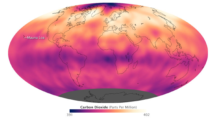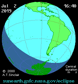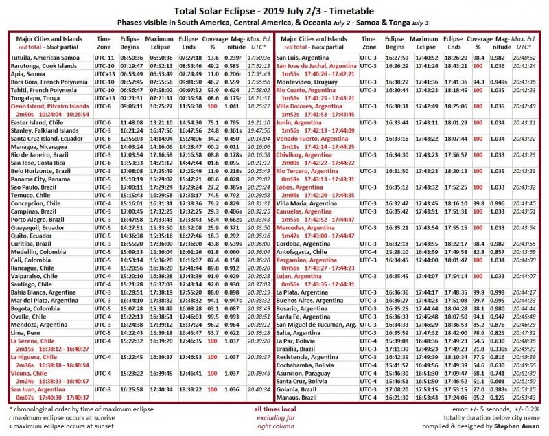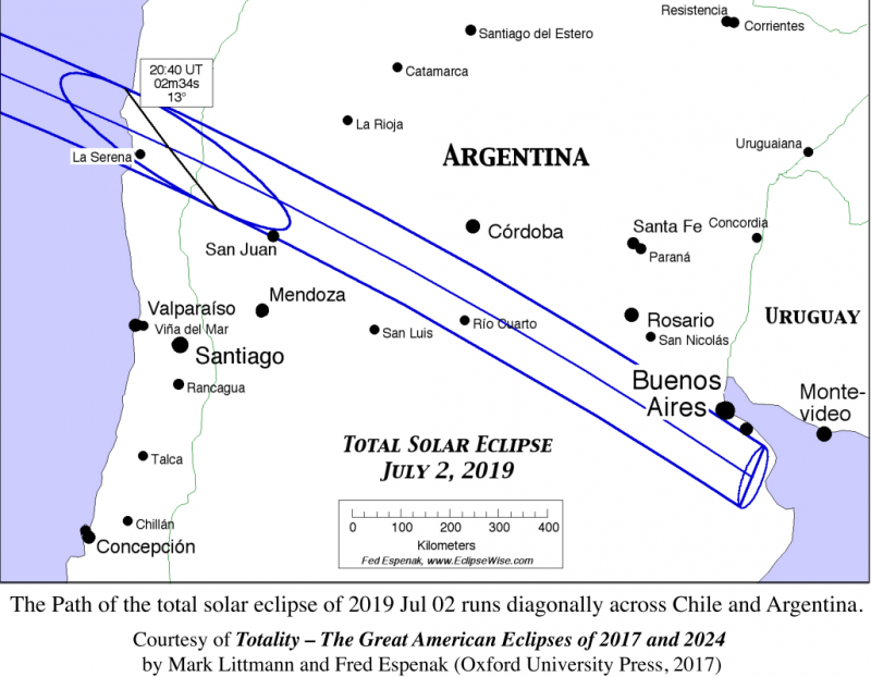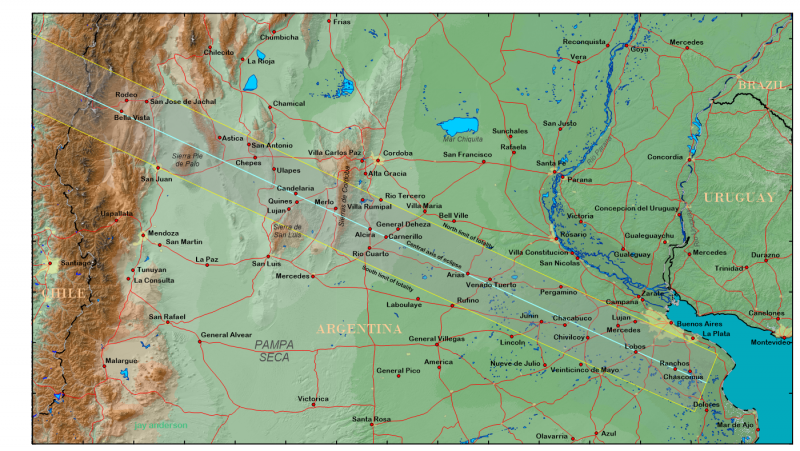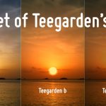
Artist’s concept comparing sunsets as viewed from Earth and from each of the 2 newly discovered planets orbiting Teegarden’s Star. Image via PHL @ UPR Arecibo.

Astronomers have confirmed over 4,000 exoplanets – planets orbiting other stars – so far, and among these are a growing number of Earth-sized worlds. Now, two more such planets have been found, orbiting one of the nearest stars to our own solar system, just 12.5 light-years away. These new planets – orbiting Teegarden’s Star – might also be potentially habitable, since both are in their star’s habitable zone.

An international team of astronomers from the University of Göttingen announced the discovery on June 18, 2019. Their peer-reviewed results were accepted in Astronomy & Astrophysics on May 14, 2019.

At 12.5 light-years away, the planets are some of the closest found so far. Astronomers have labeled them Teegarden b and c. They are now the joint fourth-nearest habitable zone exoplanets to Earth known. The Teegarden star system itself is the 24th closest to ours. According to lead author Mathias Zechmeister:

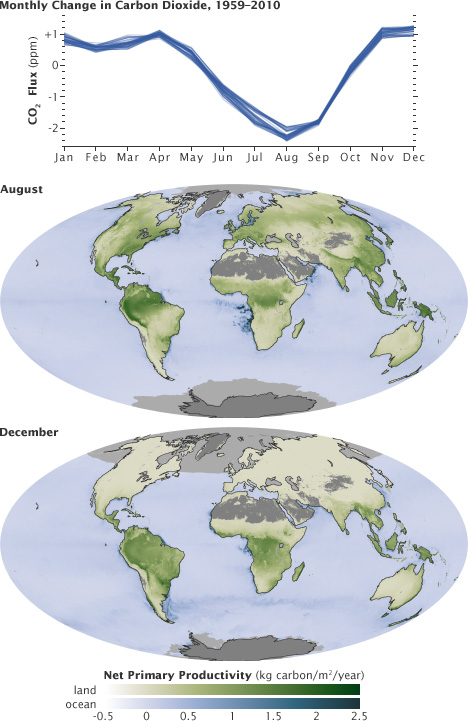
The two planets resemble the inner planets of our solar system. They are only slightly heavier than Earth and are located in the so-called habitable zone, where water can be present in liquid form.

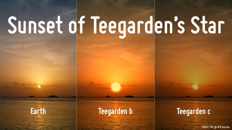
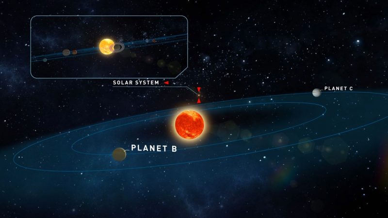
The 2 planets discovered orbiting Teegarden’s Star both reside in the habitable zone, where temperatures would allow liquid water to exist. Image via University of Göttingen, Institute for Astrophysics.

Teegarden’s Star is one of the smallest stars known, some 10 times less massive than our sun. It is also much cooler, at about 5,000 degrees Fahrenheit (2,700 degrees Celsius). Because it is so relatively cool, and thus relatively dim, Teegarden’s Star wasn’t known to astronomers until 2003, despite being so close. The star is named for the discovery team leader, Bonnard J. Teegarden, an astrophysicist at NASA’s Goddard Space Flight Center (now retired).

Teegarden’s Star is a small M-type red dwarf, and thus the habitable zone for this star is also much smaller than the one around our sun, for example. But, as it happens, both newly discovered planets orbit within this zone. That doesn’t necessarily mean there is life there, but it does show that the planets are potentially habitable, depending on other factors such as composition and atmosphere. Red dwarf stars are also notorious for emitting dangerous and powerful solar flares, which could even sometimes strip planets of their atmospheres.

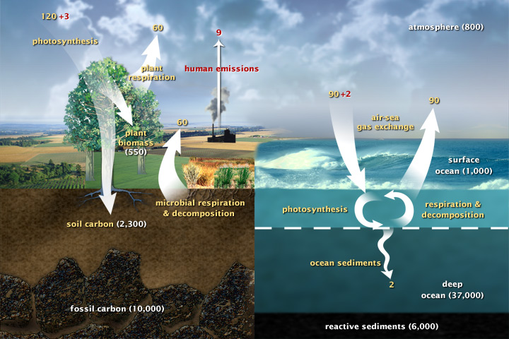
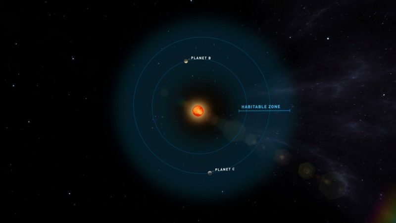
Teegarden b has been rated as “95% Earth-similar” on the Earth Similarity Index, which is based on Abel Mendez’s analysis, conducted at the Planetary Habitability Laboratory, managed by the University of Puerto Rico at Arecibo. The Earth Similarity Index is an approximation, based on known factors about a planet, but is not definitive. It serves as a guide as to how Earth-like a planet might be, but there are many factors that have to be taken into consideration. Even if the planet has water, its habitability also depends on temperature and the composition of both the planet itself and its atmosphere. As an example, this recent EarthSky story talked about potential toxic gases in a planet’s atmosphere.

According to the Earth Similarity Index, Teegarden b has a 60 percent chance of having a temperate surface environment, temperatures between 32 degrees to 122 degrees Fahrenheit (0 degrees to 50 degrees Celsius). If its atmosphere is similar to Earth’s, the surface temperature should be closer to 82 degrees F (28 degrees C). Teegarden c, farther from the star, has a 68 percent Earth Similarity Index, with only a 3 percent chance of having a warm surface temperature. The temperature is estimated to be -52 F (-47 degrees C), if the atmosphere is more similar to that of Mars. Both planets have now been added to the Planetary Habitability Laboratory’s Habitable Exoplanets Catalog.

Teegarden b and Teegarden c have now been added to the Habitable Exoplanets Catalog at the Planetary Habitability Laboratory, using the Earth Similarity Index. Image via PHL @ UPR Arecibo.

As a bonus, the astronomers also think that there might be other planets in this system. As co-author Stefan Dreizler of the University of Göttingen noted:

Many stars are apparently surrounded by systems with several planets.

Teegarden’s Star is also the smallest star where astronomers have been able to directly measure the weight of a planet. According to Ansgar Reiners, also of the University of Göttingen:

This is a great success for the Carmenes project, which was specifically designed to search for planets around the lightest stars.

The astronomers also realized something else about the Teegarden’s Star planetary system: if you were there, you would be able to look back at our own solar system and see the planets transit in front of the sun. As Reiners said:

An inhabitant of the new planets would therefore have the opportunity to view the Earth using the transit method. The new planets are the 10th and 11th discovered by the team.

Artist’s concept of the 2 new planets orbiting Teegarden’s Star. From those planets, you could see the planets in our own solar system transiting (crossing) in front of the face of our sun. Image via University of Göttingen, Institute for Astrophysics.

Graph depicting transits of planets in our solar system as seen from Teegarden’s Star. Image via University of Göttingen, Institute for Astrophysics.

This is how many exoplanets have been discovered so far, watching them transit in front of their stars, briefly blocking out some of the light coming from the star. If there were any alien astronomers at Teegarden’s star, they would be able to view the similar transits that the planets in our own solar system would make as they passed in front of the sun.

The two planets for Teegarden’s Star constitute an exciting discovery, even if we don’t fully know yet what the conditions on the planets are like. Their discovery shows, again, that smaller rocky planets like Earth are common in the galaxy (and probably the universe). This includes ones that are in the habitable zone of their stars. In our solar system, Earth is smack in the habitable zone, while Venus and Mars are near the inner and outer edges. There must be many more such planets out there, waiting to be found. How long will it be before we find one that is not only habitable, but actually inhabited with some form of life? That is still hard to tell at this point, but each discovery brings us closer to that moment.

Bottom line: The Earth-sized exoplanets orbiting Teegarden’s Star are two of the closest yet found, and at least one of them may be one of the most potentially habitable discovered so far.

Source: The CARMENES search for exoplanets around M dwarfs. Two temperate Earth-mass planet candidates around Teegarden’s Star

Via University of Göttingen

from EarthSky https://ift.tt/2YsPYdE

Artist’s concept comparing sunsets as viewed from Earth and from each of the 2 newly discovered planets orbiting Teegarden’s Star. Image via PHL @ UPR Arecibo.

Astronomers have confirmed over 4,000 exoplanets – planets orbiting other stars – so far, and among these are a growing number of Earth-sized worlds. Now, two more such planets have been found, orbiting one of the nearest stars to our own solar system, just 12.5 light-years away. These new planets – orbiting Teegarden’s Star – might also be potentially habitable, since both are in their star’s habitable zone.

An international team of astronomers from the University of Göttingen announced the discovery on June 18, 2019. Their peer-reviewed results were accepted in Astronomy & Astrophysics on May 14, 2019.

At 12.5 light-years away, the planets are some of the closest found so far. Astronomers have labeled them Teegarden b and c. They are now the joint fourth-nearest habitable zone exoplanets to Earth known. The Teegarden star system itself is the 24th closest to ours. According to lead author Mathias Zechmeister:

The two planets resemble the inner planets of our solar system. They are only slightly heavier than Earth and are located in the so-called habitable zone, where water can be present in liquid form.

The 2 planets discovered orbiting Teegarden’s Star both reside in the habitable zone, where temperatures would allow liquid water to exist. Image via University of Göttingen, Institute for Astrophysics.

Teegarden’s Star is one of the smallest stars known, some 10 times less massive than our sun. It is also much cooler, at about 5,000 degrees Fahrenheit (2,700 degrees Celsius). Because it is so relatively cool, and thus relatively dim, Teegarden’s Star wasn’t known to astronomers until 2003, despite being so close. The star is named for the discovery team leader, Bonnard J. Teegarden, an astrophysicist at NASA’s Goddard Space Flight Center (now retired).

Teegarden’s Star is a small M-type red dwarf, and thus the habitable zone for this star is also much smaller than the one around our sun, for example. But, as it happens, both newly discovered planets orbit within this zone. That doesn’t necessarily mean there is life there, but it does show that the planets are potentially habitable, depending on other factors such as composition and atmosphere. Red dwarf stars are also notorious for emitting dangerous and powerful solar flares, which could even sometimes strip planets of their atmospheres.

Teegarden b has been rated as “95% Earth-similar” on the Earth Similarity Index, which is based on Abel Mendez’s analysis, conducted at the Planetary Habitability Laboratory, managed by the University of Puerto Rico at Arecibo. The Earth Similarity Index is an approximation, based on known factors about a planet, but is not definitive. It serves as a guide as to how Earth-like a planet might be, but there are many factors that have to be taken into consideration. Even if the planet has water, its habitability also depends on temperature and the composition of both the planet itself and its atmosphere. As an example, this recent EarthSky story talked about potential toxic gases in a planet’s atmosphere.

According to the Earth Similarity Index, Teegarden b has a 60 percent chance of having a temperate surface environment, temperatures between 32 degrees to 122 degrees Fahrenheit (0 degrees to 50 degrees Celsius). If its atmosphere is similar to Earth’s, the surface temperature should be closer to 82 degrees F (28 degrees C). Teegarden c, farther from the star, has a 68 percent Earth Similarity Index, with only a 3 percent chance of having a warm surface temperature. The temperature is estimated to be -52 F (-47 degrees C), if the atmosphere is more similar to that of Mars. Both planets have now been added to the Planetary Habitability Laboratory’s Habitable Exoplanets Catalog.

Teegarden b and Teegarden c have now been added to the Habitable Exoplanets Catalog at the Planetary Habitability Laboratory, using the Earth Similarity Index. Image via PHL @ UPR Arecibo.

As a bonus, the astronomers also think that there might be other planets in this system. As co-author Stefan Dreizler of the University of Göttingen noted:

Many stars are apparently surrounded by systems with several planets.

Teegarden’s Star is also the smallest star where astronomers have been able to directly measure the weight of a planet. According to Ansgar Reiners, also of the University of Göttingen:

This is a great success for the Carmenes project, which was specifically designed to search for planets around the lightest stars.

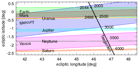
The astronomers also realized something else about the Teegarden’s Star planetary system: if you were there, you would be able to look back at our own solar system and see the planets transit in front of the sun. As Reiners said:

An inhabitant of the new planets would therefore have the opportunity to view the Earth using the transit method. The new planets are the 10th and 11th discovered by the team.

Artist’s concept of the 2 new planets orbiting Teegarden’s Star. From those planets, you could see the planets in our own solar system transiting (crossing) in front of the face of our sun. Image via University of Göttingen, Institute for Astrophysics.

Graph depicting transits of planets in our solar system as seen from Teegarden’s Star. Image via University of Göttingen, Institute for Astrophysics.

This is how many exoplanets have been discovered so far, watching them transit in front of their stars, briefly blocking out some of the light coming from the star. If there were any alien astronomers at Teegarden’s star, they would be able to view the similar transits that the planets in our own solar system would make as they passed in front of the sun.

The two planets for Teegarden’s Star constitute an exciting discovery, even if we don’t fully know yet what the conditions on the planets are like. Their discovery shows, again, that smaller rocky planets like Earth are common in the galaxy (and probably the universe). This includes ones that are in the habitable zone of their stars. In our solar system, Earth is smack in the habitable zone, while Venus and Mars are near the inner and outer edges. There must be many more such planets out there, waiting to be found. How long will it be before we find one that is not only habitable, but actually inhabited with some form of life? That is still hard to tell at this point, but each discovery brings us closer to that moment.

Bottom line: The Earth-sized exoplanets orbiting Teegarden’s Star are two of the closest yet found, and at least one of them may be one of the most potentially habitable discovered so far.

Source: The CARMENES search for exoplanets around M dwarfs. Two temperate Earth-mass planet candidates around Teegarden’s Star

Via University of Göttingen

from EarthSky https://ift.tt/2YsPYdE

6 things to know about carbon dioxide

NOAA’s Mauna Loa Observatory in Hawaii. The Mauna Loa Observatory has been measuring carbon dioxide since 1958. The remote location (high on a volcano) and scarce vegetation make it a good place to monitor carbon dioxide because it does not have much interference from local sources of the gas. (There are occasional volcanic emissions, but scientists can easily monitor and filter them out.) Mauna Loa is part of a globally distributed network of air sampling sites that measure how much carbon dioxide is in the atmosphere. Image via NOAA.

By Adam Voiland, NASA Earth Observatory

In May 2019, when atmospheric carbon dioxide reached its yearly peak, it set a record. The May average concentration of the greenhouse gas was 414.7 parts per million (ppm), as observed at NOAA’s Mauna Loa Atmospheric Baseline Observatory in Hawaii. That was the highest seasonal peak in 61 years, and the seventh consecutive year with a steep increase, according to NOAA and the Scripps Institution of Oceanography.

The broad consensus among climate scientists is that increasing concentrations of carbon dioxide in the atmosphere are causing temperatures to warm, sea levels to rise, oceans to grow more acidic, and rainstorms, droughts, floods and fires to become more severe. Here are six less widely known but interesting things to know about carbon dioxide.

Global concentrations of atmospheric carbon dioxide spike every April or May, but in 2019 the spike was bigger than usual. The dashed red line represents the monthly mean values; the black line shows the same data after the seasonal effects have been averaged out. Image via NOAA. Read more about the graph.

1. The rate of increase is accelerating.

For decades, carbon dioxide concentrations have been increasing every year. In the 1960s, Mauna Loa saw annual increases around 0.8 ppm per year. By the 1980s and 1990s, the growth rate was up to 1.5 ppm year. Now it is above 2 ppm per year. There is “abundant and conclusive evidence” that the acceleration is caused by increased emissions, according to Pieter Tans, senior scientist with NOAA’s Global Monitoring Division.

Image via NOAA/Scripps Institute of Oceanography. Read more about the chart.

2. Scientists have detailed records of atmospheric carbon dioxide that go back 800,000 years.

To understand carbon dioxide variations prior to 1958, scientists rely on ice cores. Researchers have drilled deep into icepack in Antarctica and Greenland and taken samples of ice that are thousands of years old. That old ice contains trapped air bubbles that make it possible for scientists to reconstruct past carbon dioxide levels. The video below, produced by NOAA, illustrates this data set in beautiful detail. Notice how the variations and seasonal “noise” in the observations at short time scales fade away as you look at longer time scales.

3. CO2 is not evenly distributed.

Satellite observations show carbon dioxide in the air can be somewhat patchy, with high concentrations in some places and lower concentrations in others. For instance, the map below shows carbon dioxide levels for May 2013 in the mid-troposphere, the part of the atmosphere where most weather occurs. At the time there was more carbon dioxide in the northern hemisphere because crops, grasses, and trees hadn’t greened up yet and absorbed some of the gas. The transport and distribution of CO2 throughout the atmosphere is controlled by the jet stream, large weather systems, and other large-scale atmospheric circulations. This patchiness has raised interesting questions about how carbon dioxide is transported from one part of the atmosphere to another – both horizontally and vertically.

The first space-based instrument to independently measure atmospheric carbon dioxide day and night, and under both clear and cloudy conditions over the entire globe, was the Atmospheric Infrared Sounder (AIRS) on NASA’s Aqua satellite. Read more about this world CO2 map. The OCO-2 satellite, launched in 2014, also makes global measurements of carbon dioxide, and it does so at even lower altitudes in the atmosphere than AIRS.

4. Despite the patchiness, there is still lots of mixing.

In this animation from NASA’s Scientific Visualization Studio, big plumes of carbon dioxide stream from cities in North America, Asia, and Europe. They also rise from areas with active crop fires or wildfires. Yet these plumes quickly get mixed as they rise and encounter high-altitude winds. In the visualization, reds and yellows show regions of higher than average CO2, while blues show regions lower than average. The pulsing of the data is caused by the day/night cycle of plant photosynthesis at the ground. This view highlights carbon dioxide emissions from crop fires in South America and Africa. The carbon dioxide can be transported over long distances, but notice how mountains can block the flow of the gas.

5. Carbon dioxide peaks during the Northern Hemisphere spring.

You’ll notice that there is a distinct sawtooth pattern in charts that show how carbon dioxide is changing over time. There are peaks and dips in carbon dioxide caused by seasonal changes in vegetation. Plants, trees, and crops absorb carbon dioxide, so seasons with more vegetation have lower levels of the gas. Carbon dioxide concentrations typically peak in April and May because decomposing leaves in forests in the Northern Hemisphere (particularly Canada and Russia) have been adding carbon dioxide to the air all winter, while new leaves have not yet sprouted and absorbed much of the gas. In the chart and maps below, the ebb and flow of the carbon cycle is visible by comparing the monthly changes in carbon dioxide with the globe’s net primary productivity, a measure of how much carbon dioxide vegetation consumes during photosynthesis minus the amount they release during respiration. Notice that carbon dioxide dips in Northern Hemisphere summer.

Image via NASA Earth Observatory. Read more about this image.

6. It isn’t just about what is happening in the atmosphere.

Most of Earth’s carbon – about 65,500 billion metric tons – is stored in rocks. The rest resides in the ocean, atmosphere, plants, soil, and fossil fuels. Carbon flows between each reservoir in the carbon cycle, which has slow and fast components. Any change in the cycle that shifts carbon out of one reservoir puts more carbon into other reservoirs. Any changes that put more carbon gases into the atmosphere result in warmer air temperatures. That’s why burning fossil fuels or wildfires are not the only factors determining what happens with atmospheric carbon dioxide. Things like the activity of phytoplankton, the health of the world’s forests, and the ways we change the landscapes through farming or building can play critical roles as well. Read more about the carbon cycle.

The carbon cycle. Image via NASA.

Bottom line: Facts about the greenhouse gas carbon dioxide (C02).

from EarthSky https://ift.tt/2RM4xXt

NOAA’s Mauna Loa Observatory in Hawaii. The Mauna Loa Observatory has been measuring carbon dioxide since 1958. The remote location (high on a volcano) and scarce vegetation make it a good place to monitor carbon dioxide because it does not have much interference from local sources of the gas. (There are occasional volcanic emissions, but scientists can easily monitor and filter them out.) Mauna Loa is part of a globally distributed network of air sampling sites that measure how much carbon dioxide is in the atmosphere. Image via NOAA.

By Adam Voiland, NASA Earth Observatory

In May 2019, when atmospheric carbon dioxide reached its yearly peak, it set a record. The May average concentration of the greenhouse gas was 414.7 parts per million (ppm), as observed at NOAA’s Mauna Loa Atmospheric Baseline Observatory in Hawaii. That was the highest seasonal peak in 61 years, and the seventh consecutive year with a steep increase, according to NOAA and the Scripps Institution of Oceanography.

The broad consensus among climate scientists is that increasing concentrations of carbon dioxide in the atmosphere are causing temperatures to warm, sea levels to rise, oceans to grow more acidic, and rainstorms, droughts, floods and fires to become more severe. Here are six less widely known but interesting things to know about carbon dioxide.

Global concentrations of atmospheric carbon dioxide spike every April or May, but in 2019 the spike was bigger than usual. The dashed red line represents the monthly mean values; the black line shows the same data after the seasonal effects have been averaged out. Image via NOAA. Read more about the graph.

1. The rate of increase is accelerating.

For decades, carbon dioxide concentrations have been increasing every year. In the 1960s, Mauna Loa saw annual increases around 0.8 ppm per year. By the 1980s and 1990s, the growth rate was up to 1.5 ppm year. Now it is above 2 ppm per year. There is “abundant and conclusive evidence” that the acceleration is caused by increased emissions, according to Pieter Tans, senior scientist with NOAA’s Global Monitoring Division.

Image via NOAA/Scripps Institute of Oceanography. Read more about the chart.

2. Scientists have detailed records of atmospheric carbon dioxide that go back 800,000 years.

To understand carbon dioxide variations prior to 1958, scientists rely on ice cores. Researchers have drilled deep into icepack in Antarctica and Greenland and taken samples of ice that are thousands of years old. That old ice contains trapped air bubbles that make it possible for scientists to reconstruct past carbon dioxide levels. The video below, produced by NOAA, illustrates this data set in beautiful detail. Notice how the variations and seasonal “noise” in the observations at short time scales fade away as you look at longer time scales.

3. CO2 is not evenly distributed.

Satellite observations show carbon dioxide in the air can be somewhat patchy, with high concentrations in some places and lower concentrations in others. For instance, the map below shows carbon dioxide levels for May 2013 in the mid-troposphere, the part of the atmosphere where most weather occurs. At the time there was more carbon dioxide in the northern hemisphere because crops, grasses, and trees hadn’t greened up yet and absorbed some of the gas. The transport and distribution of CO2 throughout the atmosphere is controlled by the jet stream, large weather systems, and other large-scale atmospheric circulations. This patchiness has raised interesting questions about how carbon dioxide is transported from one part of the atmosphere to another – both horizontally and vertically.

The first space-based instrument to independently measure atmospheric carbon dioxide day and night, and under both clear and cloudy conditions over the entire globe, was the Atmospheric Infrared Sounder (AIRS) on NASA’s Aqua satellite. Read more about this world CO2 map. The OCO-2 satellite, launched in 2014, also makes global measurements of carbon dioxide, and it does so at even lower altitudes in the atmosphere than AIRS.

4. Despite the patchiness, there is still lots of mixing.

In this animation from NASA’s Scientific Visualization Studio, big plumes of carbon dioxide stream from cities in North America, Asia, and Europe. They also rise from areas with active crop fires or wildfires. Yet these plumes quickly get mixed as they rise and encounter high-altitude winds. In the visualization, reds and yellows show regions of higher than average CO2, while blues show regions lower than average. The pulsing of the data is caused by the day/night cycle of plant photosynthesis at the ground. This view highlights carbon dioxide emissions from crop fires in South America and Africa. The carbon dioxide can be transported over long distances, but notice how mountains can block the flow of the gas.

5. Carbon dioxide peaks during the Northern Hemisphere spring.

You’ll notice that there is a distinct sawtooth pattern in charts that show how carbon dioxide is changing over time. There are peaks and dips in carbon dioxide caused by seasonal changes in vegetation. Plants, trees, and crops absorb carbon dioxide, so seasons with more vegetation have lower levels of the gas. Carbon dioxide concentrations typically peak in April and May because decomposing leaves in forests in the Northern Hemisphere (particularly Canada and Russia) have been adding carbon dioxide to the air all winter, while new leaves have not yet sprouted and absorbed much of the gas. In the chart and maps below, the ebb and flow of the carbon cycle is visible by comparing the monthly changes in carbon dioxide with the globe’s net primary productivity, a measure of how much carbon dioxide vegetation consumes during photosynthesis minus the amount they release during respiration. Notice that carbon dioxide dips in Northern Hemisphere summer.

Image via NASA Earth Observatory. Read more about this image.

6. It isn’t just about what is happening in the atmosphere.

Most of Earth’s carbon – about 65,500 billion metric tons – is stored in rocks. The rest resides in the ocean, atmosphere, plants, soil, and fossil fuels. Carbon flows between each reservoir in the carbon cycle, which has slow and fast components. Any change in the cycle that shifts carbon out of one reservoir puts more carbon into other reservoirs. Any changes that put more carbon gases into the atmosphere result in warmer air temperatures. That’s why burning fossil fuels or wildfires are not the only factors determining what happens with atmospheric carbon dioxide. Things like the activity of phytoplankton, the health of the world’s forests, and the ways we change the landscapes through farming or building can play critical roles as well. Read more about the carbon cycle.

The carbon cycle. Image via NASA.

Bottom line: Facts about the greenhouse gas carbon dioxide (C02).

from EarthSky https://ift.tt/2RM4xXt

Skeptical Science New Climate Research for Week #26, 2019

Welcome to another heaping helping of research publications related to climate change drivers and mechanisms, the effects of climate change and how we might yet grope our way into systems approaches to dealing with the mess we're making, despite ourselves.

52 items this week, derived from some 277 abstracts/articles emerging from our raw feed filter and evaluated for salience and impact.

Skeptical Science was founded to help people wade out of the swamp of misinformation found in public discussions of climate change. A perennial feature and expedient go-to of science denier arguments has been the seemingly paradoxical behavior of sea ice around Antarctica, with ice coverage stubbornly holding  and even increasing slightly for the past few decades even as the rest of the ocean/atmosphere system and dependencies showed obvious, growing signs of stress. There are good reasons for this seeming conundrum, but perhaps we're encountering limits to those controls. NASA GSFC researcher Claire Parkinson sums up recent details in the PNAS article A 40-y record reveals gradual Antarctic sea ice increases followed by decreases at rates far exceeding the rates in the Arctic.  For another twist on blasts from the past, see A Positive Iris Feedback: Insights from Climate Simulations with Temperature Sensitive Cloud-Rain Conversion

Other papers of interest:

Public policy and human cognition encounter climate change

Communicating Climate Change: Probabilistic Expressions and Concrete Events

The urban governance of climate change adaptation in least-developed African countries and in small cities: the engagement of local decision-makers in Dar es Salaam, Tanzania, and Karonga, Malawi

Technology transfer and adoption for smallholder climate change adaptation: opportunities and challenges

Climate information services for adaptation: what does it mean to know the context?

Increasing Local Salience of Climate Change: The Un-tapped Impact of the Media-science Interface

Going Global: Climate Change Discourse in Presidential Communications

Climate risk assessments and management options for redevelopment of the Parliamentary Complex in Samoa, South Pacific (OA)

Health consequences of climate change in Bangladesh: An overview of the evidence, knowledge gaps and challenges

Biology and climate change

C3 plants converge on a universal relationship between leaf maximum carboxylation rate and chlorophyll content

Using Respiration Quotients to Track Changing Sources of Soil Respiration Seasonally and with Experimental Warming (OA)

Effectiveness of vegetated patches as Green Infrastructure in mitigating urban heat island effects during a heatwave event in the city of Melbourne (OA)

Disentangling how climate change can affect an aquatic food web by combining multiple experimental approaches

Biological interactions: The overlooked aspects of marine climate change refugia

Strong photosynthetic acclimation and enhanced water‐use efficiency in grassland functional groups persist over 21 years of CO2 enrichment, independent of nitrogen supply

Physical science of climate change

Changes in temperature seasonality in China: human influences and internal variability

Moist static energy budget analysis of tropical cyclone intensification in high-resolution climate models

AN ANALOG APPROACH FOR WEATHER ESTIMATION USING CLIMATE PROJECTIONS AND REANALYSIS DATA (Why is this this title in all-caps? We DON"T KNOW!)

A Positive Iris Feedback: Insights from Climate Simulations with Temperature Sensitive Cloud-Rain Conversion

Reassessing the effect of cloud type on Earth’s energy balance in the age of active spaceborne observations. Part I: Top-of-atmosphere and surface

The dominant role of snow/ice albedo feedback strengthened by black carbon in the enhanced warming over the Himalayas

Thickness of the divide and flank of the West Antarctic Ice Sheet through the last deglaciation

The sub-adiabatic model as a concept for evaluating the representation and radiative effects of low-level clouds in a high-resolution atmospheric model (OA)

A reconstruction of warm-water inflow to Upernavik Isstrøm since 1925 CE and its relation to glacier retreat

Global database and model on dissolved carbon in soil solution (OA)

Contrail cirrus radiative forcing for future air traffic (OA)

Sea ice volume variability and water temperature in the Greenland Sea (OA)

West Greenland ice sheet retreat history reveals elevated precipitation during the Holocene thermal maximum (OA)

Observed transport decline at 47°N, western Atlantic

Climate‐sensitive controls on large spring emissions of CH4 and CO2 from northern lakes

(below is a perfect collision of public policy and research)

Framework for high‐end estimates of sea‐level rise for stakeholder applications

Ambiguity in the land‐use component of mitigation contributions towards the Paris Agreement goals

Controls on the width of tropical precipitation and its contraction under global warming

Model Structure and Climate Data Uncertainty in Historical Simulations of the Terrestrial Carbon Cycle (1850–2014)

Regional differences in sea level rise between the Mid‐Atlantic Bight and the South Atlantic Bight: Is the Gulf Stream to blame?

The effects of anthropogenic land‐use changes on climate in China driven by global socioeconomic and emission scenarios

Geographical distribution of thermometers gives the appearance of lower historical global warming

The effect of QBO phase on the atmospheric response to projected Arctic sea‐ice loss in early winter

Long term measurements of methane ebullition from thaw ponds

Multi-tracer study of gas trapping in an East Antarctic ice core

The double ITCZ syndrome in GCMs: A coupled feedback problem among convection, clouds, atmospheric and ocean circulations

Comments on “Comparing the current and early 20th century warm periods in China” by Soon W., R. Connolly, M. Connolly et al.

Temporal evolution of precipitation-based climate change indices across India: contrast between pre- and post-1975 features

Global and regional impacts of climate change at different levels of global temperature increase (OA)

Non‐stationarity of summer temperature extremes in Texas

Assessment of CMIP5 multimodel mean for the historical climate of Africa

Negative feedback processes following drainage slow down permafrost degradation

Multi‐century trends to wetter winters and drier summers in the England and Wales precipitation series explained by observational and sampling bias in early records

Intensified inundation shifts a freshwater wetland from a CO2 sink to a source

Strong photosynthetic acclimation and enhanced water‐use efficiency in grassland functional groups persist over 21 years of CO2 enrichment, independent of nitrogen supply

Accumulation of soil carbon under elevated CO2 unaffected by warming and drought

Climate change impacts on Canadian yields of spring wheat, canola and maize for global warming levels of 1.5 °C, 2.0 °C, 2.5 °C and 3.0 °C

Changes in risk of extreme weather events in Europe

Nonstationary joint probability analysis of extreme marine variables to assess design water levels at the shoreline in a changing climate

The previous edition of New Climate Research may be found here.

from Skeptical Science https://ift.tt/2RRQ0td

Welcome to another heaping helping of research publications related to climate change drivers and mechanisms, the effects of climate change and how we might yet grope our way into systems approaches to dealing with the mess we're making, despite ourselves.

52 items this week, derived from some 277 abstracts/articles emerging from our raw feed filter and evaluated for salience and impact.

Skeptical Science was founded to help people wade out of the swamp of misinformation found in public discussions of climate change. A perennial feature and expedient go-to of science denier arguments has been the seemingly paradoxical behavior of sea ice around Antarctica, with ice coverage stubbornly holding  and even increasing slightly for the past few decades even as the rest of the ocean/atmosphere system and dependencies showed obvious, growing signs of stress. There are good reasons for this seeming conundrum, but perhaps we're encountering limits to those controls. NASA GSFC researcher Claire Parkinson sums up recent details in the PNAS article A 40-y record reveals gradual Antarctic sea ice increases followed by decreases at rates far exceeding the rates in the Arctic.  For another twist on blasts from the past, see A Positive Iris Feedback: Insights from Climate Simulations with Temperature Sensitive Cloud-Rain Conversion

Other papers of interest:

Public policy and human cognition encounter climate change

Communicating Climate Change: Probabilistic Expressions and Concrete Events

The urban governance of climate change adaptation in least-developed African countries and in small cities: the engagement of local decision-makers in Dar es Salaam, Tanzania, and Karonga, Malawi

Technology transfer and adoption for smallholder climate change adaptation: opportunities and challenges

Climate information services for adaptation: what does it mean to know the context?

Increasing Local Salience of Climate Change: The Un-tapped Impact of the Media-science Interface

Going Global: Climate Change Discourse in Presidential Communications

Climate risk assessments and management options for redevelopment of the Parliamentary Complex in Samoa, South Pacific (OA)

Health consequences of climate change in Bangladesh: An overview of the evidence, knowledge gaps and challenges

Biology and climate change

C3 plants converge on a universal relationship between leaf maximum carboxylation rate and chlorophyll content

Using Respiration Quotients to Track Changing Sources of Soil Respiration Seasonally and with Experimental Warming (OA)

Effectiveness of vegetated patches as Green Infrastructure in mitigating urban heat island effects during a heatwave event in the city of Melbourne (OA)

Disentangling how climate change can affect an aquatic food web by combining multiple experimental approaches

Biological interactions: The overlooked aspects of marine climate change refugia

Strong photosynthetic acclimation and enhanced water‐use efficiency in grassland functional groups persist over 21 years of CO2 enrichment, independent of nitrogen supply

Physical science of climate change

Changes in temperature seasonality in China: human influences and internal variability

Moist static energy budget analysis of tropical cyclone intensification in high-resolution climate models

AN ANALOG APPROACH FOR WEATHER ESTIMATION USING CLIMATE PROJECTIONS AND REANALYSIS DATA (Why is this this title in all-caps? We DON"T KNOW!)

A Positive Iris Feedback: Insights from Climate Simulations with Temperature Sensitive Cloud-Rain Conversion

Reassessing the effect of cloud type on Earth’s energy balance in the age of active spaceborne observations. Part I: Top-of-atmosphere and surface

The dominant role of snow/ice albedo feedback strengthened by black carbon in the enhanced warming over the Himalayas

Thickness of the divide and flank of the West Antarctic Ice Sheet through the last deglaciation

The sub-adiabatic model as a concept for evaluating the representation and radiative effects of low-level clouds in a high-resolution atmospheric model (OA)

A reconstruction of warm-water inflow to Upernavik Isstrøm since 1925 CE and its relation to glacier retreat

Global database and model on dissolved carbon in soil solution (OA)

Contrail cirrus radiative forcing for future air traffic (OA)

Sea ice volume variability and water temperature in the Greenland Sea (OA)

West Greenland ice sheet retreat history reveals elevated precipitation during the Holocene thermal maximum (OA)

Observed transport decline at 47°N, western Atlantic

Climate‐sensitive controls on large spring emissions of CH4 and CO2 from northern lakes

(below is a perfect collision of public policy and research)

Framework for high‐end estimates of sea‐level rise for stakeholder applications

Ambiguity in the land‐use component of mitigation contributions towards the Paris Agreement goals

Controls on the width of tropical precipitation and its contraction under global warming

Model Structure and Climate Data Uncertainty in Historical Simulations of the Terrestrial Carbon Cycle (1850–2014)

Regional differences in sea level rise between the Mid‐Atlantic Bight and the South Atlantic Bight: Is the Gulf Stream to blame?

The effects of anthropogenic land‐use changes on climate in China driven by global socioeconomic and emission scenarios

Geographical distribution of thermometers gives the appearance of lower historical global warming

The effect of QBO phase on the atmospheric response to projected Arctic sea‐ice loss in early winter

Long term measurements of methane ebullition from thaw ponds

Multi-tracer study of gas trapping in an East Antarctic ice core

The double ITCZ syndrome in GCMs: A coupled feedback problem among convection, clouds, atmospheric and ocean circulations

Comments on “Comparing the current and early 20th century warm periods in China” by Soon W., R. Connolly, M. Connolly et al.

Temporal evolution of precipitation-based climate change indices across India: contrast between pre- and post-1975 features

Global and regional impacts of climate change at different levels of global temperature increase (OA)

Non‐stationarity of summer temperature extremes in Texas

Assessment of CMIP5 multimodel mean for the historical climate of Africa

Negative feedback processes following drainage slow down permafrost degradation

Multi‐century trends to wetter winters and drier summers in the England and Wales precipitation series explained by observational and sampling bias in early records

Intensified inundation shifts a freshwater wetland from a CO2 sink to a source

Strong photosynthetic acclimation and enhanced water‐use efficiency in grassland functional groups persist over 21 years of CO2 enrichment, independent of nitrogen supply

Accumulation of soil carbon under elevated CO2 unaffected by warming and drought

Climate change impacts on Canadian yields of spring wheat, canola and maize for global warming levels of 1.5 °C, 2.0 °C, 2.5 °C and 3.0 °C

Changes in risk of extreme weather events in Europe

Nonstationary joint probability analysis of extreme marine variables to assess design water levels at the shoreline in a changing climate

The previous edition of New Climate Research may be found here.

from Skeptical Science https://ift.tt/2RRQ0td

July guide to the bright planets

Click the name of a planet to learn more about its visibility in July 2019: Venus, Jupiter, Saturn, Mars and Mercury.

On the morning of July 1 – as seen from around the world – the waning moon is near bright Venus. This very bright planet is also very low in your eastern dawn sky and thus not easy to see. Read more.

Venus, the brightest planet, looms low in the east before sunrise in early July 2019. Day by day, Venus sinks closer to the sunrise, so this world must contend with the sun’s glare throughout this month. However, if you’re in just the right spot in South America, you can watch Venus pop into view during the total eclipse of the sun on July 2, 2019.

In early July, at mid-northern latitudes, Venus rises less than an hour before sunrise. By the month’s end, that’ll taper to about 20 minutes.

At temperate latitudes in the Southern Hemisphere, Venus rises about 50 minutes before sunup in early July. By the month’s end that’ll decrease to about 10 minutes.

In other words – for all of Earth – Venus will disappear from our sky in early July, assuming you’re looking with your eye alone.

What is happening to Venus? Where’s it going? It’s now fleeing ahead of Earth in the race of the planets around the sun. On August 14, 2019, Venus will reach superior conjunction, when it will be behind the sun as seen from Earth. At that point, it’ll transition from the morning to evening sky. Most of us will begin to see Venus as a bright evening “star” in September.

Coming soon! The young evening crescent swings by the planets Mercury and Mars on July 3 and 4, 2019. They’ll be hard to see in the afterglow of sunset; you’ll definitely want your binoculars. Read more.

Mercury starts off the month rather close to Mars on the sky’s dome. Your best chance of catching them is early in the month, when these two worlds are out for a maximum amount of time after sunset. On July 3 and 4, 2019, the young crescent moon will be in the vicinity of Mercury and Mars. But all three celestial bodies – the moon, Mercury and Mars – will have to contend with the glow of sunset, so have binoculars handy.

Click here for recommended sky almanacs providing you with the setting times for Mercury and Mars in your sky.

Day by day, however, these two worlds sink closer to the sunset, with Mercury doing so at a much faster pace than Mars. Mercury moves faster than Mars in orbit, and it moves faster in our sky as well. That’s why the early stargazers named Mercury for their fleet-footed messenger god.

Mercury will meet up with the sun, at inferior conjunction, on July 21, 2019. In the days before and after Mercury’s July 21 conjunction, skilled observers with telescopes will be able to view the planet as a thin crescent world. July 21 will also mark Mercury’s transition out of the evening sky and into the morning sky.

Mars will meet up with the sun, at superior conjunction, on September 2, 2019. For at least six weeks or so on either side of that date, Mars will be absent from our sky, lost in the sun’s glare.

By the way, at this upcoming conjunction, Mercury will swing to the south of the sun’s disk as seen from Earth. But when Mercury reaches its next inferior conjunction on November 11, 2019, the innermost planet will swing directly in front of the sun, to stage a transit of Mercury. Transits of Mercury happen more frequently than transits of Venus; they happen 13 or 14 times per century. The last transit of Mercury happened on May 9, 2016, and – after the one on this upcoming November 11 – the next Mercury transit won’t be until November 13, 2032.

Here’s a superior conjunction. The planet sweeps behind the sun as seen from Earth. Image via COSMOS.

Here’s an inferior conjunction. The planet sweeps between the Earth and sun. As seen from Earth, only Venus and Mercury can have inferior conjunctions. Image via COSMOS.

On the evenings of July 12, 13 and 14, 2019, watch for the bright waxing gibbous moon to swing by the giant planet Jupiter. Read more.

Jupiter – the second-brightest planet after Venus – reigns supreme in the July 2019 nighttime sky. Venus is mostly lost in the glare of sunrise throughout July. Jupiter, on the other hand, pops out in the eastern sky at dusk and stays out nearly all night. Jupiter is very bright, brighter than any star. Still not sure? See the moon in Jupiter’s vicinity for several days, centered on or near July 13.

Jupiter’s yearly opposition was June 10, 2019, when this planet lit up the night sky from dusk until dawn. Now, since Jupiter is already in the east when night begins, it doesn’t make it until dawn. From around the world in early July, Jupiter sets about 1 1/2 hours before sunrise (approximate beginning of astronomical twilight). By the end of the month, Jupiter will set beneath the southwest horizon about two hours before the start of astronomical twilight.

Click here to find out when astronomical twilight comes to your sky, remembering to check the astronomical twilight box.

That bright ruddy star rather close to Jupiter on our sky’s dome this year is Antares, the Heart of the Scorpion in the constellation Scorpius. Throughout 2019, Jupiter can be seen to “wander” relative to this zodiac star. In other words, in the first three months of 2019, Jupiter was traveling eastward, away from Antares. But starting on April 10, 2019, Jupiter appeared to reverse course, moving toward Antares. For four months (April 10 to August 11, 2019), Jupiter will be traveling in retrograde (or westward), closing the gap between itself and the star Antares. Midway through this retrograde – on June 10, 2019 – Jupiter reached opposition.

Can’t find Saturn? The almost-full moon pairs up with it as darkness falls on July 15, 2019. Read more.

Saturn reaches opposition on July 9, 2019. At opposition, Saturn rises in the east around sunset, climbs highest up for the night at midnight (midway between sunset and sunrise) and sets in the west around sunrise. Opposition happens when Earth in its orbit swings between the sun and Saturn. Our two worlds are close now, and Saturn, in turn, shines at its brightest best in Earth’s sky.

Watch for the bright moon to couple up with Saturn on or near July 15, as shown on the sky chart above. If you’re in just the right spot in South America, you can actually watch the moon occult (cover over) Saturn on the night of July 15-16, 2019.

Don’t mistake Saturn for the more brilliant planet Jupiter. At nightfall and early evening in July 2019, Saturn shines well below Jupiter and quite close to the southeast horizon. Saturn, although somewhat brighter than a 1st-magnitude star, pales in contrast to the king planet. Jupiter, the fourth-brightest celestial object after the sun, moon and Venus, respectively, outshines Saturn by some 11 times.

In early July 2019, Saturn rises about 1/2 hour after sunset. At opposition on July 9, Saturn rises as the sun sets.

By the month’s end, Saturn comes up roughly 1 1/2 hours before sunset, though the exact figure varies somewhat, depending on your latitude.

Viewing Saturn’s rings soon? Read me 1st

Here’s an opposition. It happens when Earth flies between a planet and the sun. This happens yearly for most of the outer planets (except Mars). Note that the image is not to scale. Saturn is about 9.5 times the Earth’s distance from the sun. Earth goes between the sun and Saturn once a year, 2 weeks later each year. Image via Heavens Above.

What do we mean by bright planet? By bright planet, we mean any solar system planet that is easily visible without an optical aid and that has been watched by our ancestors since time immemorial. In their outward order from the sun, the five bright planets are Mercury, Venus, Mars, Jupiter and Saturn. These planets actually do appear bright in our sky. They are typically as bright as – or brighter than – the brightest stars. Plus, these relatively nearby worlds tend to shine with a steadier light than the distant, twinkling stars. You can spot them, and come to know them as faithful friends, if you try.

Skywatcher, by Predrag Agatonovic.

Bottom line: In July 2019, two planets – Jupiter and Saturn – are easy to see throughout the month. They both come out at nightfall and are out nearly all night long. Mercury and Mars lurk low in the afterglow of sunset, whereas Venus sits deeply in the glare of morning dawn. Click here for recommended almanacs; they can help you know when the planets rise and set in your sky.

Don’t miss anything. Subscribe to EarthSky News by email

Visit EarthSky’s Best Places to Stargaze, and recommend a place we can all enjoy. Zoom out for worldwide map.

Help EarthSky keep going! Donate now.

Post your planet photos at EarthSky Community Photos

from EarthSky https://ift.tt/1YD00CF

Click the name of a planet to learn more about its visibility in July 2019: Venus, Jupiter, Saturn, Mars and Mercury.

On the morning of July 1 – as seen from around the world – the waning moon is near bright Venus. This very bright planet is also very low in your eastern dawn sky and thus not easy to see. Read more.

Venus, the brightest planet, looms low in the east before sunrise in early July 2019. Day by day, Venus sinks closer to the sunrise, so this world must contend with the sun’s glare throughout this month. However, if you’re in just the right spot in South America, you can watch Venus pop into view during the total eclipse of the sun on July 2, 2019.

In early July, at mid-northern latitudes, Venus rises less than an hour before sunrise. By the month’s end, that’ll taper to about 20 minutes.

At temperate latitudes in the Southern Hemisphere, Venus rises about 50 minutes before sunup in early July. By the month’s end that’ll decrease to about 10 minutes.

In other words – for all of Earth – Venus will disappear from our sky in early July, assuming you’re looking with your eye alone.

What is happening to Venus? Where’s it going? It’s now fleeing ahead of Earth in the race of the planets around the sun. On August 14, 2019, Venus will reach superior conjunction, when it will be behind the sun as seen from Earth. At that point, it’ll transition from the morning to evening sky. Most of us will begin to see Venus as a bright evening “star” in September.

Coming soon! The young evening crescent swings by the planets Mercury and Mars on July 3 and 4, 2019. They’ll be hard to see in the afterglow of sunset; you’ll definitely want your binoculars. Read more.

Mercury starts off the month rather close to Mars on the sky’s dome. Your best chance of catching them is early in the month, when these two worlds are out for a maximum amount of time after sunset. On July 3 and 4, 2019, the young crescent moon will be in the vicinity of Mercury and Mars. But all three celestial bodies – the moon, Mercury and Mars – will have to contend with the glow of sunset, so have binoculars handy.

Click here for recommended sky almanacs providing you with the setting times for Mercury and Mars in your sky.

Day by day, however, these two worlds sink closer to the sunset, with Mercury doing so at a much faster pace than Mars. Mercury moves faster than Mars in orbit, and it moves faster in our sky as well. That’s why the early stargazers named Mercury for their fleet-footed messenger god.

Mercury will meet up with the sun, at inferior conjunction, on July 21, 2019. In the days before and after Mercury’s July 21 conjunction, skilled observers with telescopes will be able to view the planet as a thin crescent world. July 21 will also mark Mercury’s transition out of the evening sky and into the morning sky.

Mars will meet up with the sun, at superior conjunction, on September 2, 2019. For at least six weeks or so on either side of that date, Mars will be absent from our sky, lost in the sun’s glare.

By the way, at this upcoming conjunction, Mercury will swing to the south of the sun’s disk as seen from Earth. But when Mercury reaches its next inferior conjunction on November 11, 2019, the innermost planet will swing directly in front of the sun, to stage a transit of Mercury. Transits of Mercury happen more frequently than transits of Venus; they happen 13 or 14 times per century. The last transit of Mercury happened on May 9, 2016, and – after the one on this upcoming November 11 – the next Mercury transit won’t be until November 13, 2032.

Here’s a superior conjunction. The planet sweeps behind the sun as seen from Earth. Image via COSMOS.

Here’s an inferior conjunction. The planet sweeps between the Earth and sun. As seen from Earth, only Venus and Mercury can have inferior conjunctions. Image via COSMOS.

On the evenings of July 12, 13 and 14, 2019, watch for the bright waxing gibbous moon to swing by the giant planet Jupiter. Read more.

Jupiter – the second-brightest planet after Venus – reigns supreme in the July 2019 nighttime sky. Venus is mostly lost in the glare of sunrise throughout July. Jupiter, on the other hand, pops out in the eastern sky at dusk and stays out nearly all night. Jupiter is very bright, brighter than any star. Still not sure? See the moon in Jupiter’s vicinity for several days, centered on or near July 13.

Jupiter’s yearly opposition was June 10, 2019, when this planet lit up the night sky from dusk until dawn. Now, since Jupiter is already in the east when night begins, it doesn’t make it until dawn. From around the world in early July, Jupiter sets about 1 1/2 hours before sunrise (approximate beginning of astronomical twilight). By the end of the month, Jupiter will set beneath the southwest horizon about two hours before the start of astronomical twilight.

Click here to find out when astronomical twilight comes to your sky, remembering to check the astronomical twilight box.

That bright ruddy star rather close to Jupiter on our sky’s dome this year is Antares, the Heart of the Scorpion in the constellation Scorpius. Throughout 2019, Jupiter can be seen to “wander” relative to this zodiac star. In other words, in the first three months of 2019, Jupiter was traveling eastward, away from Antares. But starting on April 10, 2019, Jupiter appeared to reverse course, moving toward Antares. For four months (April 10 to August 11, 2019), Jupiter will be traveling in retrograde (or westward), closing the gap between itself and the star Antares. Midway through this retrograde – on June 10, 2019 – Jupiter reached opposition.

Can’t find Saturn? The almost-full moon pairs up with it as darkness falls on July 15, 2019. Read more.

Saturn reaches opposition on July 9, 2019. At opposition, Saturn rises in the east around sunset, climbs highest up for the night at midnight (midway between sunset and sunrise) and sets in the west around sunrise. Opposition happens when Earth in its orbit swings between the sun and Saturn. Our two worlds are close now, and Saturn, in turn, shines at its brightest best in Earth’s sky.

Watch for the bright moon to couple up with Saturn on or near July 15, as shown on the sky chart above. If you’re in just the right spot in South America, you can actually watch the moon occult (cover over) Saturn on the night of July 15-16, 2019.

Don’t mistake Saturn for the more brilliant planet Jupiter. At nightfall and early evening in July 2019, Saturn shines well below Jupiter and quite close to the southeast horizon. Saturn, although somewhat brighter than a 1st-magnitude star, pales in contrast to the king planet. Jupiter, the fourth-brightest celestial object after the sun, moon and Venus, respectively, outshines Saturn by some 11 times.

In early July 2019, Saturn rises about 1/2 hour after sunset. At opposition on July 9, Saturn rises as the sun sets.

By the month’s end, Saturn comes up roughly 1 1/2 hours before sunset, though the exact figure varies somewhat, depending on your latitude.

Viewing Saturn’s rings soon? Read me 1st

Here’s an opposition. It happens when Earth flies between a planet and the sun. This happens yearly for most of the outer planets (except Mars). Note that the image is not to scale. Saturn is about 9.5 times the Earth’s distance from the sun. Earth goes between the sun and Saturn once a year, 2 weeks later each year. Image via Heavens Above.

What do we mean by bright planet? By bright planet, we mean any solar system planet that is easily visible without an optical aid and that has been watched by our ancestors since time immemorial. In their outward order from the sun, the five bright planets are Mercury, Venus, Mars, Jupiter and Saturn. These planets actually do appear bright in our sky. They are typically as bright as – or brighter than – the brightest stars. Plus, these relatively nearby worlds tend to shine with a steadier light than the distant, twinkling stars. You can spot them, and come to know them as faithful friends, if you try.

Skywatcher, by Predrag Agatonovic.

Bottom line: In July 2019, two planets – Jupiter and Saturn – are easy to see throughout the month. They both come out at nightfall and are out nearly all night long. Mercury and Mars lurk low in the afterglow of sunset, whereas Venus sits deeply in the glare of morning dawn. Click here for recommended almanacs; they can help you know when the planets rise and set in your sky.

Don’t miss anything. Subscribe to EarthSky News by email

Visit EarthSky’s Best Places to Stargaze, and recommend a place we can all enjoy. Zoom out for worldwide map.

Help EarthSky keep going! Donate now.

Post your planet photos at EarthSky Community Photos

from EarthSky https://ift.tt/1YD00CF

Why no eclipse every full and new moon?

Total lunar eclipse composite image by Fred Espenak.

A lunar eclipse happens when the Earth, sun and moon align in space, with Earth between the sun and moon. At such times, Earth’s shadow falls on the full moon, darkening the moon’s face and – at mid-eclipse – usually turning it a coppery red.

A solar eclipse happens at the opposite phase of the moon – new moon – when the moon passes between the sun and Earth.

Why aren’t there eclipses at every full and new moon?

The moon takes about a month to orbit around the Earth. If the moon orbited in the same plane as the ecliptic – Earth’s orbital plane – we would have a minimum of two eclipses every month. There’d be an eclipse of the moon at every full moon. And, one fortnight (approximately two weeks) later there’d be an eclipse of the sun at new moon for a total of at least 24 eclipses every year.

But the moon’s orbit is inclined to Earth’s orbit by about five degrees. Twice a month the moon intersects the ecliptic – Earth’s orbital plane – at points called nodes. If the moon is going from south to north in its orbit, it’s called an ascending node. If the moon is going from north to south, it’s a descending node. If the full moon or new moon is appreciably close to one of these nodes, then an eclipse is not only possible – but inevitable.

Coming up…Total lunar eclipse of July 2, 2019

Visit EarthSky’s Best Places to Stargaze to find an eclipse-viewing location

Post your eclipse photo to EarthSky Community Photos

The plane of the moon’s orbit is inclined at 5 degrees to the ecliptic (Earth’s orbital plane). In this diagram, the ecliptic is portrayed as the sun’s apparent annual path through the constellations of the zodiac. The moon’s orbit intersects the ecliptic at two points called nodes (N1 and N2).

Solar and lunar eclipses always come in pairs, with one following the other in a period of one fortnight (approximately two weeks). For example, in January 2019, the descending node partial solar eclipse on January 6 was followed by the ascending node total lunar eclipse on January 21.

Then exactly six lunar months (six new moons) after the descending node partial solar eclipse on January 6, there’s an ascending node total solar eclipse on July 2. One fortnight after this ascending node July 2 total solar eclipse, there will be a descending node partial lunar eclipse on July 16.

Then exactly six lunar months (six new moons) after the ascending node total solar eclipse of July 2, the final eclipse of 2019 will present a descending node annular solar eclipse on December 26. One fortnight later, the first eclipse of 2020 will fall on January 10, 2020, to feature an ascending node and hard-to-see penumbral lunar eclipse.

Read more: Dates of solar and lunar eclipses in 2019

More often than not, two eclipses – one solar and one lunar – occur in one eclipse season, a period lasting approximately 34 to 35 days. Sometimes, though, when the initial eclipse happens sufficiently early in the eclipse season, there can be three eclipses in one eclipse season (two solar and one lunar, or two lunar and one solar). The last time this happened was in 2018 (solar/lunar/solar), and the next time will be in 2020 (lunar/solar/lunar).

Read more: How often are there 3 eclipses in a month?

This year, in 2019, the middle of the eclipse season happens on January 17, July 10 and December 30. At the middle of an eclipse season, which recurs in periods of about 173 days, the lunar nodes are in exact alignment with the Earth and sun.

The video below explains why a pair of eclipses happens when the new moon and full moon are closely aligned with the lunar nodes.

There might be some unfamiliar words in this video, including ecliptic and node. The ecliptic is the plane of Earth’s orbit around the sun. The moon’s orbit is inclined to the plane of the ecliptic. The nodes are the two points where the moon’s orbit and the ecliptic intersect.

Relative to the moon’s nodes, the moon’s phases recur about 30 degrees farther eastward (counterclockwise) along the zodiac each month. So the next pair of eclipses won’t be forthcoming for nearly another six calendar months (6 x 30 degrees = 180 degrees), to fall on December 26, 2019, and January 10, 2020.

Node passages of the moon: 2001 to 2100

Phases of the moon: 2001 to 2100

The following new moon and full moon happen again nearly 30 degrees farther eastward as measured by the constellations of the zodiac in about 29.5 days. But the moon returns to its node a good two days earlier than that, or in about 27.2 days. After the eclipses of July 2 and 16, 2019, it’ll be a waning crescent moon (not a new moon) that crosses the moon’s ascending node on July 30, 2019, and a waxing gibbous moon (not a full moon) that crosses the moon’s descending node on August 12, 2019.

A heliocentric or sun-centered view of eclipses in 2019. Earth-moon orbit shown at new and full moon dates. Sizes of Earth, moon, sun very exaggerated. The plane of the moon’s orbit is in blue, with the dark-blue half to the north of the ecliptic, and the light-blue half to the south of the ecliptic. The line dividing the dark-blue and light-blue sides depicts the line of nodes. There’s an eclipse if the moon is full or new when it is in or near the ecliptic or sun-Earth plane. This year there are 5 eclipses, instead of the most usual 4, because a 3rd eclipse season begins before the end of the year. Illustration via Guy Ottewell.

Even though the moon’s orbit is inclined to that of Earth – and even though there’s not an eclipse with every new and full moon – there are more eclipses than you might think.

There are from four to seven eclipses every year. Some are solar, some are lunar, some are total, and some are partial. All are marvelous to behold – a reminder that we live on a planet – a chance to experience falling in line with great worlds in space!

Photo via pizzodisevo.

Bottom line: There’s no eclipse at every full moon and new moon because the moon’s orbit is inclined to Earth’s orbit by about five degrees. Most of the time, the sun, Earth and moon don’t line up precisely enough to cause an eclipse. But sometimes, more often than you might expect, they do!

Donate: It means the world to us

EarthSky lunar calendars are cool! They make great gifts. Order now. Going fast!

from EarthSky https://ift.tt/2XfOwtU

Total lunar eclipse composite image by Fred Espenak.

A lunar eclipse happens when the Earth, sun and moon align in space, with Earth between the sun and moon. At such times, Earth’s shadow falls on the full moon, darkening the moon’s face and – at mid-eclipse – usually turning it a coppery red.

A solar eclipse happens at the opposite phase of the moon – new moon – when the moon passes between the sun and Earth.

Why aren’t there eclipses at every full and new moon?

The moon takes about a month to orbit around the Earth. If the moon orbited in the same plane as the ecliptic – Earth’s orbital plane – we would have a minimum of two eclipses every month. There’d be an eclipse of the moon at every full moon. And, one fortnight (approximately two weeks) later there’d be an eclipse of the sun at new moon for a total of at least 24 eclipses every year.

But the moon’s orbit is inclined to Earth’s orbit by about five degrees. Twice a month the moon intersects the ecliptic – Earth’s orbital plane – at points called nodes. If the moon is going from south to north in its orbit, it’s called an ascending node. If the moon is going from north to south, it’s a descending node. If the full moon or new moon is appreciably close to one of these nodes, then an eclipse is not only possible – but inevitable.

Coming up…Total lunar eclipse of July 2, 2019

Visit EarthSky’s Best Places to Stargaze to find an eclipse-viewing location

Post your eclipse photo to EarthSky Community Photos

The plane of the moon’s orbit is inclined at 5 degrees to the ecliptic (Earth’s orbital plane). In this diagram, the ecliptic is portrayed as the sun’s apparent annual path through the constellations of the zodiac. The moon’s orbit intersects the ecliptic at two points called nodes (N1 and N2).

Solar and lunar eclipses always come in pairs, with one following the other in a period of one fortnight (approximately two weeks). For example, in January 2019, the descending node partial solar eclipse on January 6 was followed by the ascending node total lunar eclipse on January 21.

Then exactly six lunar months (six new moons) after the descending node partial solar eclipse on January 6, there’s an ascending node total solar eclipse on July 2. One fortnight after this ascending node July 2 total solar eclipse, there will be a descending node partial lunar eclipse on July 16.

Then exactly six lunar months (six new moons) after the ascending node total solar eclipse of July 2, the final eclipse of 2019 will present a descending node annular solar eclipse on December 26. One fortnight later, the first eclipse of 2020 will fall on January 10, 2020, to feature an ascending node and hard-to-see penumbral lunar eclipse.

Read more: Dates of solar and lunar eclipses in 2019

More often than not, two eclipses – one solar and one lunar – occur in one eclipse season, a period lasting approximately 34 to 35 days. Sometimes, though, when the initial eclipse happens sufficiently early in the eclipse season, there can be three eclipses in one eclipse season (two solar and one lunar, or two lunar and one solar). The last time this happened was in 2018 (solar/lunar/solar), and the next time will be in 2020 (lunar/solar/lunar).

Read more: How often are there 3 eclipses in a month?

This year, in 2019, the middle of the eclipse season happens on January 17, July 10 and December 30. At the middle of an eclipse season, which recurs in periods of about 173 days, the lunar nodes are in exact alignment with the Earth and sun.

The video below explains why a pair of eclipses happens when the new moon and full moon are closely aligned with the lunar nodes.

There might be some unfamiliar words in this video, including ecliptic and node. The ecliptic is the plane of Earth’s orbit around the sun. The moon’s orbit is inclined to the plane of the ecliptic. The nodes are the two points where the moon’s orbit and the ecliptic intersect.

Relative to the moon’s nodes, the moon’s phases recur about 30 degrees farther eastward (counterclockwise) along the zodiac each month. So the next pair of eclipses won’t be forthcoming for nearly another six calendar months (6 x 30 degrees = 180 degrees), to fall on December 26, 2019, and January 10, 2020.

Node passages of the moon: 2001 to 2100

Phases of the moon: 2001 to 2100

The following new moon and full moon happen again nearly 30 degrees farther eastward as measured by the constellations of the zodiac in about 29.5 days. But the moon returns to its node a good two days earlier than that, or in about 27.2 days. After the eclipses of July 2 and 16, 2019, it’ll be a waning crescent moon (not a new moon) that crosses the moon’s ascending node on July 30, 2019, and a waxing gibbous moon (not a full moon) that crosses the moon’s descending node on August 12, 2019.

A heliocentric or sun-centered view of eclipses in 2019. Earth-moon orbit shown at new and full moon dates. Sizes of Earth, moon, sun very exaggerated. The plane of the moon’s orbit is in blue, with the dark-blue half to the north of the ecliptic, and the light-blue half to the south of the ecliptic. The line dividing the dark-blue and light-blue sides depicts the line of nodes. There’s an eclipse if the moon is full or new when it is in or near the ecliptic or sun-Earth plane. This year there are 5 eclipses, instead of the most usual 4, because a 3rd eclipse season begins before the end of the year. Illustration via Guy Ottewell.

Even though the moon’s orbit is inclined to that of Earth – and even though there’s not an eclipse with every new and full moon – there are more eclipses than you might think.

There are from four to seven eclipses every year. Some are solar, some are lunar, some are total, and some are partial. All are marvelous to behold – a reminder that we live on a planet – a chance to experience falling in line with great worlds in space!

Photo via pizzodisevo.

Bottom line: There’s no eclipse at every full moon and new moon because the moon’s orbit is inclined to Earth’s orbit by about five degrees. Most of the time, the sun, Earth and moon don’t line up precisely enough to cause an eclipse. But sometimes, more often than you might expect, they do!

Donate: It means the world to us

EarthSky lunar calendars are cool! They make great gifts. Order now. Going fast!

from EarthSky https://ift.tt/2XfOwtU

South American solar eclipse on July 2

Above: Beverley Sinclair’s photo of the solar eclipse on August 21, 2017, highlighting the diamond ring effect.

A total eclipse of the sun is coming to the South American countries of Chile and Argentina in the late afternoon hours of July 2, 2019. This is the first total solar eclipse since the great American total solar eclipse of August 21, 2017.

We refer to the map below. Outside the narrow path of totality (in blue) that swings over the South Pacific Ocean and southern South America, a much broader swath of the Pacific, South America and southern Central America sits beneath the moon’s penumbral shadow, to undergo a partial eclipse of the sun. It’ll be an exceedingly shallow solar eclipse for southern Central America, however. Be sure to use proper eye protection any time the sun is not eclipsed or in any stage of a partial eclipse (even when it’s over 99 percent but less than 100 percent eclipsed)!

Top 7 tips for safe solar eclipse viewing

The narrow dark blue corridor depicts the path of totality; you must be on that path to see a total eclipse. The broader swath shows varying degrees of a partial solar eclipse. The numbers (0.80 to 0.20) indicate how much of the sun’s diameter is covered over by the moon. The total eclipse will start at sunrise, at left, and – some 2 2/3 hours later – it’ll end at sunset over eastern Argentina. The path of totality is approximately 7,000 miles (11,200 km) long. The maximum path width is 125 miles (201 km).

An animated version of the above map whereby the small black dot depicts totality. The large gray circle shows the region of a partial eclipse of the sun.

Unless you’re on a cruise ship, or perhaps an airplane, you can only watch the total solar eclipse from Chile or Argentina in South America. Oneo, a small and uninhabited atoll of the Pitcairn Islands, is the only Pacific island where the total solar eclipse is visible, starting at 10:24 a.m. local time (18:24 Universal Time). Totality lasts for 2 minutes and 53 seconds. Numerous Pacific islands, on the other hand, can observe a partial solar eclipse – but, once again, we stress the need for proper eye protection.

View larger. | Stephen Aman in Orlando, Florida, kindly provided this chart of eclipse times for all major cities and islands that lie in its path. Thank you, Stephen!

We expect eclipse chasers to flock to the big cities of Santiago, Chile, and Buenos Aires, Argentina, in their quest to witness the most spectacular of natural wonders, a total eclipse of the sun. It’s been said that on a scale of one to ten, a total solar eclipse rates a million! After seeing a total solar eclipse for the first time in Wyoming on August 21, 2017, I have to agree with the assessment. If you live in South America and are within traveling distance of totality, by all means take the trip. It’s an experience that’ll live with you for the rest of your days.

View larger. Zooming in on the path of totality going through Chile and Argentina via Mark Littmann and Fred Espenak.

As evident on the map above, Santiago, Chile, lies to the south of the total eclipse path, whereas Buenos Aires, Argentina, sits at the northern edge. We give the eclipse times in local time for Santiago, Chile, and Buenos Aires, Argentina, plus two cities within the total eclipse path: La Serena, Chile, and Rio Cuarto, Argentina.

Local eclipse times:

Santiago, Chile
Partial solar eclipse begins: 4:21 p.m local time
Maximum eclipse (sun’s disk 92.1 percent covered over): 4:37 p.m. local time
Partial solar eclipse ends: 7:44 p.m. local time

Buenos Aires, Argentina
Partial solar eclipse begins: 4:36 p.m. local time
Maximum eclipse (sun’s disk 99.7 percent covered over): 5:44 p.m. local time
Sunset (eclipse still in process): 5:51 p.m. local time

La Serena, Chile
Partial solar eclipse begins: 3:23 p.m.local time
Total solar eclipse begins: 4:38:13 p.m. local time
Maximum eclipse: 4:39:23 p.m. local time
Total solar eclipse ends: 4:40:31 p.m. local time
Partial solar eclipse ends 5:47 p.m. local time

Rio Cuarto, Argentina
Partial solar eclipse begins: 4:31 p.m. local time
Total solar eclipse begins: 5:41:26 p.m. local time
Maximum eclipse: 5:42:26 p.m. local time
Total solar eclipse ends: 5:43:26 p.m local time
Sunset (eclipse still in process): 6:22 p.m. local time

Resources:

Solar eclipse calculator via EclipseWise

Eclipse information via TimeandDate

If you want to find out when (or if) this eclipse happens in your sky, click on either one of the above links or this Google map.

View larger. Map of total eclipse path through Argentina via Eclipsophile. Along the central line of the total eclipse path, totality lasts for about 2 minutes at the beginning and end points, and around 4 1/2 minutes around the midpoint. Click here for details.

What causes a solar eclipse?

A solar eclipse is only possible at new moon, when the moon in its orbit swings between Earth and the sun. Then the moon blocks out the solar disk, either partially or totally, as viewed from a portion of the Earth’s surface. More often than not, however, no solar eclipse happens at new moon, because the new moon swings to the north or south of the sun. Despite having 13 new moons in 2019, there are only three solar eclipses:

January 6, 2019: partial solar eclipse
July 2, 2019: total solar eclipse
December 26, 2019: annular solar eclipse

This year, in 2019, we have 13 new moons and 3 solar eclipses (P = partial, T = total and A = annular). We also have 12 full moons and 2 lunar eclipses (t = total and p = partial). Moon phase table via Astropixels.

Read more: Why no eclipse at every full and new moon?

During the course of one year, the new moon swings anywhere from 5 degrees (10 moon diameters) north of the ecliptic (Earth’s orbital plane) to 5 degrees south of the ecliptic. Yet a solar eclipse can only happen when the new moon is appreciably close to the ecliptic. After the year’s first solar eclipse on January 6, 2019, the following five new moons swung too far south of the ecliptic for a solar eclipse to take place. After the year’s second solar eclipse on July 2, 2019, the following five new moons will swing too far north of the ecliptic to feature a solar eclipse.

A = total solar eclipse, B = annular eclipse and C = partial solar eclipse

The upcoming total solar eclipse on July 2, 2019, depends on more than the fortuitous alignment of the new moon with the Earth and sun. For a total solar eclipse to occur, the angular diameter of the moon has to exceed that of the sun. During this eclipse, the new moon comes considerably closer than its average distance from Earth. Yet, at the same time, the Earth is only a few days shy of reaching its farthest point from the sun.

The closer moon makes the new moon appear larger, whereas the more distant sun makes the sun appear smaller. Because the new moon looms larger than the sun in Earth’s sky, the moon totally covers over the solar disk during the total solar eclipse of July 2, 2019.

Annular solar eclipse – called a “ring of fire” eclipse – captured by photographer Geoff Sims on May 10, 2013. Used with permission.

Six lunar months (six new moons) after the total solar eclipse on July 2, 2019, the year’s final solar eclipse will fall on December 26, 2019. But this time around, the December 2019 new moon will be about 10,000 miles (16,000 km) farther than the new moon of July 2019. Also, the sun will be about 3 million miles (5 million km) closer than it was in July 2019. On December 26, 2019, the smaller new moon won’t be able to totally cover over the larger solar disk, so a ring of sunshine will surround the new moon silhouette, to showcase an annular eclipse of the sun.

The total solar eclipse on July 2, 2019, will be the last total eclipse of the sun to grace Earth’s sky until December 14, 2020. Hard to believe, but the path of totality on both July 2, 2019, and December 14, 2020, will sweep over Chile and Argentina, to give these lucky South American residents a total solar eclipse for two years in a row.

Bottom line: A total eclipse of the sun is coming to the South American countries of Chile and Argentina in the late afternoon hours on July 2, 2019.

from EarthSky https://ift.tt/2Xif3vn

Above: Beverley Sinclair’s photo of the solar eclipse on August 21, 2017, highlighting the diamond ring effect.

A total eclipse of the sun is coming to the South American countries of Chile and Argentina in the late afternoon hours of July 2, 2019. This is the first total solar eclipse since the great American total solar eclipse of August 21, 2017.

We refer to the map below. Outside the narrow path of totality (in blue) that swings over the South Pacific Ocean and southern South America, a much broader swath of the Pacific, South America and southern Central America sits beneath the moon’s penumbral shadow, to undergo a partial eclipse of the sun. It’ll be an exceedingly shallow solar eclipse for southern Central America, however. Be sure to use proper eye protection any time the sun is not eclipsed or in any stage of a partial eclipse (even when it’s over 99 percent but less than 100 percent eclipsed)!

Top 7 tips for safe solar eclipse viewing

The narrow dark blue corridor depicts the path of totality; you must be on that path to see a total eclipse. The broader swath shows varying degrees of a partial solar eclipse. The numbers (0.80 to 0.20) indicate how much of the sun’s diameter is covered over by the moon. The total eclipse will start at sunrise, at left, and – some 2 2/3 hours later – it’ll end at sunset over eastern Argentina. The path of totality is approximately 7,000 miles (11,200 km) long. The maximum path width is 125 miles (201 km).

An animated version of the above map whereby the small black dot depicts totality. The large gray circle shows the region of a partial eclipse of the sun.

Unless you’re on a cruise ship, or perhaps an airplane, you can only watch the total solar eclipse from Chile or Argentina in South America. Oneo, a small and uninhabited atoll of the Pitcairn Islands, is the only Pacific island where the total solar eclipse is visible, starting at 10:24 a.m. local time (18:24 Universal Time). Totality lasts for 2 minutes and 53 seconds. Numerous Pacific islands, on the other hand, can observe a partial solar eclipse – but, once again, we stress the need for proper eye protection.

View larger. | Stephen Aman in Orlando, Florida, kindly provided this chart of eclipse times for all major cities and islands that lie in its path. Thank you, Stephen!

We expect eclipse chasers to flock to the big cities of Santiago, Chile, and Buenos Aires, Argentina, in their quest to witness the most spectacular of natural wonders, a total eclipse of the sun. It’s been said that on a scale of one to ten, a total solar eclipse rates a million! After seeing a total solar eclipse for the first time in Wyoming on August 21, 2017, I have to agree with the assessment. If you live in South America and are within traveling distance of totality, by all means take the trip. It’s an experience that’ll live with you for the rest of your days.

View larger. Zooming in on the path of totality going through Chile and Argentina via Mark Littmann and Fred Espenak.

As evident on the map above, Santiago, Chile, lies to the south of the total eclipse path, whereas Buenos Aires, Argentina, sits at the northern edge. We give the eclipse times in local time for Santiago, Chile, and Buenos Aires, Argentina, plus two cities within the total eclipse path: La Serena, Chile, and Rio Cuarto, Argentina.

Local eclipse times:

Santiago, Chile
Partial solar eclipse begins: 4:21 p.m local time
Maximum eclipse (sun’s disk 92.1 percent covered over): 4:37 p.m. local time
Partial solar eclipse ends: 7:44 p.m. local time

Buenos Aires, Argentina
Partial solar eclipse begins: 4:36 p.m. local time
Maximum eclipse (sun’s disk 99.7 percent covered over): 5:44 p.m. local time
Sunset (eclipse still in process): 5:51 p.m. local time

La Serena, Chile
Partial solar eclipse begins: 3:23 p.m.local time
Total solar eclipse begins: 4:38:13 p.m. local time
Maximum eclipse: 4:39:23 p.m. local time
Total solar eclipse ends: 4:40:31 p.m. local time
Partial solar eclipse ends 5:47 p.m. local time

Rio Cuarto, Argentina
Partial solar eclipse begins: 4:31 p.m. local time
Total solar eclipse begins: 5:41:26 p.m. local time
Maximum eclipse: 5:42:26 p.m. local time
Total solar eclipse ends: 5:43:26 p.m local time
Sunset (eclipse still in process): 6:22 p.m. local time

Resources:

Solar eclipse calculator via EclipseWise

Eclipse information via TimeandDate

If you want to find out when (or if) this eclipse happens in your sky, click on either one of the above links or this Google map.

View larger. Map of total eclipse path through Argentina via Eclipsophile. Along the central line of the total eclipse path, totality lasts for about 2 minutes at the beginning and end points, and around 4 1/2 minutes around the midpoint. Click here for details.

What causes a solar eclipse?

A solar eclipse is only possible at new moon, when the moon in its orbit swings between Earth and the sun. Then the moon blocks out the solar disk, either partially or totally, as viewed from a portion of the Earth’s surface. More often than not, however, no solar eclipse happens at new moon, because the new moon swings to the north or south of the sun. Despite having 13 new moons in 2019, there are only three solar eclipses:

January 6, 2019: partial solar eclipse
July 2, 2019: total solar eclipse
December 26, 2019: annular solar eclipse

This year, in 2019, we have 13 new moons and 3 solar eclipses (P = partial, T = total and A = annular). We also have 12 full moons and 2 lunar eclipses (t = total and p = partial). Moon phase table via Astropixels.

Read more: Why no eclipse at every full and new moon?

During the course of one year, the new moon swings anywhere from 5 degrees (10 moon diameters) north of the ecliptic (Earth’s orbital plane) to 5 degrees south of the ecliptic. Yet a solar eclipse can only happen when the new moon is appreciably close to the ecliptic. After the year’s first solar eclipse on January 6, 2019, the following five new moons swung too far south of the ecliptic for a solar eclipse to take place. After the year’s second solar eclipse on July 2, 2019, the following five new moons will swing too far north of the ecliptic to feature a solar eclipse.

A = total solar eclipse, B = annular eclipse and C = partial solar eclipse

The upcoming total solar eclipse on July 2, 2019, depends on more than the fortuitous alignment of the new moon with the Earth and sun. For a total solar eclipse to occur, the angular diameter of the moon has to exceed that of the sun. During this eclipse, the new moon comes considerably closer than its average distance from Earth. Yet, at the same time, the Earth is only a few days shy of reaching its farthest point from the sun.

The closer moon makes the new moon appear larger, whereas the more distant sun makes the sun appear smaller. Because the new moon looms larger than the sun in Earth’s sky, the moon totally covers over the solar disk during the total solar eclipse of July 2, 2019.

Annular solar eclipse – called a “ring of fire” eclipse – captured by photographer Geoff Sims on May 10, 2013. Used with permission.

Six lunar months (six new moons) after the total solar eclipse on July 2, 2019, the year’s final solar eclipse will fall on December 26, 2019. But this time around, the December 2019 new moon will be about 10,000 miles (16,000 km) farther than the new moon of July 2019. Also, the sun will be about 3 million miles (5 million km) closer than it was in July 2019. On December 26, 2019, the smaller new moon won’t be able to totally cover over the larger solar disk, so a ring of sunshine will surround the new moon silhouette, to showcase an annular eclipse of the sun.

The total solar eclipse on July 2, 2019, will be the last total eclipse of the sun to grace Earth’s sky until December 14, 2020. Hard to believe, but the path of totality on both July 2, 2019, and December 14, 2020, will sweep over Chile and Argentina, to give these lucky South American residents a total solar eclipse for two years in a row.

Bottom line: A total eclipse of the sun is coming to the South American countries of Chile and Argentina in the late afternoon hours on July 2, 2019.

from EarthSky https://ift.tt/2Xif3vn

NASA has a plan to knock an asteroid off course

NASA’s Deep Impact spacecraft struck a 4-mile-wide (6-km-wide) comet – called Tempel 1 – on July 4, 2005. This image was acquired 67 seconds after impact. Image via ESA.

In the past several decades, astronomers have waked up to the reality that asteroids orbiting our sun do sometimes strike the Earth. It’s now know that the relatively little ones strike fairly often, mostly disintegrating in Earth’s protective atmosphere, and/or falling into the ocean. But larger asteroids have been known to pierce Earth’s atmosphere as well, such as the one that entered over Chelyabinsk, Russia, in 2013, causing a shock wave that broke windows in several Russian cities. At present, astronomers do not expect any large, world-destroying asteroids to be on a collision course with Earth, in the foreseeable future. But smaller asteroids – those capable of causing destruction on a regional or city-wide scale, for example – are possible. And what if we learned that one was headed our way while there was still time to try to avert the collision? Could we deflect it? How?

Astronomers have been meeting and seriously talking about what might be needed to deflect an asteroid for at least a couple of decades. Those talks have evolved into action; NASA’s DART mission is planned to launch in 2021, with the goal of ramming an asteroid in 2022, and testing the asteroid’s response. Afterwards, if all goes as planned, an ESA mission called Hera – now currently under study – will also visit the asteroid, gathering more detailed information. A February 4, 2019, statement from ESA explained:

The target of [both DART and Hera] is a double asteroid system, called Didymos, which will come a comparatively close 11 million km (about 7 million miles) to Earth in 2022. The 800-meter-diameter main body (about 2,600 feet) is orbited by a 160-meter-diameter moon (about 525 feet), informally called ‘Didymoon’.

Hera manager Ian Carnelli said in an email to EarthSky that both DART and Hera fall under the framework of what scientists call the Asteroid Impact and Deflection Assessment, or AIDA. Carnelli wrote:

Our Hera and Dart mission teams are fully functional and coordinating this joint experiment. An AIDA workshop is planned in September 2019 in Rome. The original ESA part of the mission, called AIM, did not receive full funding. ESA has therefore re-worked the mission (now called Hera) and optimized for reaching Didymos after DART impact, to complete the experiment by 2026.

DART is currently planned to launch in 2021. Hera would follow a few years after DART’s impact. ESA explained:

… Hera will follow up with a detailed post-impact survey that will turn this grand-scale experiment into a well-understood and repeatable planetary defense technique.

Read more: ESA plans to visit the double asteroid, too

View larger. | DART mission profile. Illustration via ESA.

ESA also said the Hera mission will be the first spacecraft to explore a binary asteroid system – the Didymos pair. Also, the moon Didymoon will be the smallest asteroid ever visited by a spacecraft. It is about the same size as the Great Pyramid of Giza. Carnelli commented:

Such a binary asteroid system is the perfect testbed for a planetary defense experiment but is also an entirely new environment for asteroid investigations. Although binaries make up 15 percent of all known asteroids, they have never been explored before, and we anticipate many surprises.

Check out the scale chart below – prepared by the Planetary Society – of all asteroids and comets so far surveyed by spacecraft. On this chart, the larger Didymos asteroid would form a modest dot, with its smaller moonlet struggling to make a single pixel.

View larger. | The Planetary Society created this comparison chart of all the asteroids and comets visited so far by spacecraft. On this chart, the larger Didymos asteroid would form a dot, with Didymoon struggling to make a single pixel. Image via Planetary Society/ESA.

ESA said Didymoon’s small size was one reason it was chosen for a pioneering planetary defense experiment. As it happens, this little asteroid moonlet is also in the riskiest class of near-Earth asteroids because of its size: larger bodies can more easily be tracked, smaller bodies will burn up or do limited damage, while a Didymoon-sized impactor could devastate an entire region of our planet.

Read more about the Hera mission from ESA, and the DART mission from NASA, or check out the video below:

Bottom line: In what’s being called humankind’s 1st planetary defense test, space scientists are planning to send a spacecraft to a double asteroid – Didymos and its tiny moon – and crash it into the moon in attempt to change its orbit.

Via ESA

EarthSky lunar calendars are cool! They make great gifts. Order now.

from EarthSky https://ift.tt/2YmJzkp

NASA’s Deep Impact spacecraft struck a 4-mile-wide (6-km-wide) comet – called Tempel 1 – on July 4, 2005. This image was acquired 67 seconds after impact. Image via ESA.

In the past several decades, astronomers have waked up to the reality that asteroids orbiting our sun do sometimes strike the Earth. It’s now know that the relatively little ones strike fairly often, mostly disintegrating in Earth’s protective atmosphere, and/or falling into the ocean. But larger asteroids have been known to pierce Earth’s atmosphere as well, such as the one that entered over Chelyabinsk, Russia, in 2013, causing a shock wave that broke windows in several Russian cities. At present, astronomers do not expect any large, world-destroying asteroids to be on a collision course with Earth, in the foreseeable future. But smaller asteroids – those capable of causing destruction on a regional or city-wide scale, for example – are possible. And what if we learned that one was headed our way while there was still time to try to avert the collision? Could we deflect it? How?

Astronomers have been meeting and seriously talking about what might be needed to deflect an asteroid for at least a couple of decades. Those talks have evolved into action; NASA’s DART mission is planned to launch in 2021, with the goal of ramming an asteroid in 2022, and testing the asteroid’s response. Afterwards, if all goes as planned, an ESA mission called Hera – now currently under study – will also visit the asteroid, gathering more detailed information. A February 4, 2019, statement from ESA explained:

The target of [both DART and Hera] is a double asteroid system, called Didymos, which will come a comparatively close 11 million km (about 7 million miles) to Earth in 2022. The 800-meter-diameter main body (about 2,600 feet) is orbited by a 160-meter-diameter moon (about 525 feet), informally called ‘Didymoon’.

Hera manager Ian Carnelli said in an email to EarthSky that both DART and Hera fall under the framework of what scientists call the Asteroid Impact and Deflection Assessment, or AIDA. Carnelli wrote:

Our Hera and Dart mission teams are fully functional and coordinating this joint experiment. An AIDA workshop is planned in September 2019 in Rome. The original ESA part of the mission, called AIM, did not receive full funding. ESA has therefore re-worked the mission (now called Hera) and optimized for reaching Didymos after DART impact, to complete the experiment by 2026.

DART is currently planned to launch in 2021. Hera would follow a few years after DART’s impact. ESA explained:

… Hera will follow up with a detailed post-impact survey that will turn this grand-scale experiment into a well-understood and repeatable planetary defense technique.

Read more: ESA plans to visit the double asteroid, too

View larger. | DART mission profile. Illustration via ESA.

ESA also said the Hera mission will be the first spacecraft to explore a binary asteroid system – the Didymos pair. Also, the moon Didymoon will be the smallest asteroid ever visited by a spacecraft. It is about the same size as the Great Pyramid of Giza. Carnelli commented:

Such a binary asteroid system is the perfect testbed for a planetary defense experiment but is also an entirely new environment for asteroid investigations. Although binaries make up 15 percent of all known asteroids, they have never been explored before, and we anticipate many surprises.

Check out the scale chart below – prepared by the Planetary Society – of all asteroids and comets so far surveyed by spacecraft. On this chart, the larger Didymos asteroid would form a modest dot, with its smaller moonlet struggling to make a single pixel.

View larger. | The Planetary Society created this comparison chart of all the asteroids and comets visited so far by spacecraft. On this chart, the larger Didymos asteroid would form a dot, with Didymoon struggling to make a single pixel. Image via Planetary Society/ESA.

ESA said Didymoon’s small size was one reason it was chosen for a pioneering planetary defense experiment. As it happens, this little asteroid moonlet is also in the riskiest class of near-Earth asteroids because of its size: larger bodies can more easily be tracked, smaller bodies will burn up or do limited damage, while a Didymoon-sized impactor could devastate an entire region of our planet.

Read more about the Hera mission from ESA, and the DART mission from NASA, or check out the video below:

Bottom line: In what’s being called humankind’s 1st planetary defense test, space scientists are planning to send a spacecraft to a double asteroid – Didymos and its tiny moon – and crash it into the moon in attempt to change its orbit.

Via ESA

EarthSky lunar calendars are cool! They make great gifts. Order now.

from EarthSky https://ift.tt/2YmJzkp

ESA will head for the double asteroid, too

Take three minutes to watch astrophysicist and Queen guitarist Brian May tell the story of the European Space Agency’s (ESA’s) planned Hera mission, tentatively slated for 2026. Following NASA’s DART mission, ESA’s Hera mission also plans to visit a double asteroid system. The larger asteroid is named Didymos. This system is typical of the thousands that pose an impact risk to our planet, and even the smaller of the two little asteroids – the asteroid moon – would be big enough to destroy an entire city if it were to collide with Earth.

In 2022, NASA will crash its DART spacecraft into the Didymos system’s smaller asteroid, which is known as Didymoon. A few years later, Hera will come in to map the resulting impact crater and measure the asteroid’s mass. Hera will carry two CubeSats on board, which will be able to fly close to the asteroid’s surface, carrying out crucial scientific studies before touching down.

The Hera mission will be presented to an ESA meeting this November, where Europe’s space ministers will make a final decision on flying the mission.

Read more: NASA has a plan to knock an asteroid off course

Didymos is a binary asteroid. The primary body (at right) has a diameter of around half a mile (780 meters). The Didymoon secondary body (at left) has a diameter of around 525 feet (160 meters) and revolves around the primary at a distance of around .75 miles (1.2 km) in about 12 hours. Image via ESA.

Bottom line: Video narrated by Brian May explains ESA’s Hera mission to the Didymos asteroid system.

Via ESA

from EarthSky https://ift.tt/2IXyml0

Take three minutes to watch astrophysicist and Queen guitarist Brian May tell the story of the European Space Agency’s (ESA’s) planned Hera mission, tentatively slated for 2026. Following NASA’s DART mission, ESA’s Hera mission also plans to visit a double asteroid system. The larger asteroid is named Didymos. This system is typical of the thousands that pose an impact risk to our planet, and even the smaller of the two little asteroids – the asteroid moon – would be big enough to destroy an entire city if it were to collide with Earth.

In 2022, NASA will crash its DART spacecraft into the Didymos system’s smaller asteroid, which is known as Didymoon. A few years later, Hera will come in to map the resulting impact crater and measure the asteroid’s mass. Hera will carry two CubeSats on board, which will be able to fly close to the asteroid’s surface, carrying out crucial scientific studies before touching down.

The Hera mission will be presented to an ESA meeting this November, where Europe’s space ministers will make a final decision on flying the mission.

Read more: NASA has a plan to knock an asteroid off course

Didymos is a binary asteroid. The primary body (at right) has a diameter of around half a mile (780 meters). The Didymoon secondary body (at left) has a diameter of around 525 feet (160 meters) and revolves around the primary at a distance of around .75 miles (1.2 km) in about 12 hours. Image via ESA.

Bottom line: Video narrated by Brian May explains ESA’s Hera mission to the Didymos asteroid system.

Via ESA

from EarthSky https://ift.tt/2IXyml0