Come to know the Summer Triangle

We in the Northern Hemisphere can see the Summer Triangle for part of the night at any time of the year. But seeing it in summer is the most fun! As suggested by its name, the Summer Triangle is most prominent during the summer season, for us at mid-northern latitudes. Seeing the Summer Triangle again and again on summer nights is a deep pleasure that adds to the enjoyment of this season. So, as dusk deepens into night on a warm June or July night, look eastward for this great star pattern … not a constellation, but instead an asterism made of three bright stars in three different constellations.

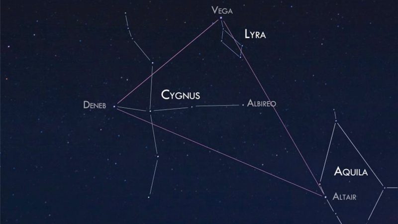
It’s difficult to convey the huge size of the Summer Triangle. At nightfall in northern summer, look for the brightest star in your eastern sky. That’s Vega, the brightest star in the constellation Lyra the Harp.

Look to the lower left of Vega for another bright star – Deneb, the brightest in the constellation Cygnus the Swan and the third brightest in the Summer Triangle. An outstretched hand at arm’s length approximates the distance from Vega to Deneb.

Look to the lower right of Vega to locate the Summer Triangle’s second brightest star. That’s Altair, the brightest star in the constellation Aquila the Eagle. A ruler held at arm’s length fills the gap between these two stars.

The Summer Triangle, as captured and composed by our friend Susan Gies Jensen in Odessa, Washington.

Summer Triangle as a road map to the Milky Way. If you’re lucky enough to be under a dark starry sky on a moonless night, you’ll see the great swath of stars known as the Milky Way passing in between the Summer Triangle stars Vega and Altair. The star Deneb bobs in the middle of this river of stars that passes through the Summer Triangle, and arcs across the sky. Although every star that you see with the unaided eye is actually a member of our Milky Way galaxy, often the term Milky Way refers to the cross-sectional view of the galactic disk, whereby innumerable far-off suns congregate into a cloudy trail of stars.

Once you master the Summer Triangle, you can always locate the Milky Way on a clear, dark night. How about making the most of a dark summer night to explore this band of stars – this starlit boulevard abounding with celestial delights? Use binoculars to reel in the gossamer beauty of it all, the haunting nebulae and star clusters of a midsummer night’s dream!

Some see the Summer Triangle as a great big “V” for vacation, with Altair marking the point of the “V.” In summer, the Summer Triangle appears in the east at nightfall, high overhead after midnight and in the west at dawn. All night long on a summer night, the stars of the Summer Triangle – as if school kids on vacation – waltz amidst the streetlights of the Milky Way galaxy.

Enjoying EarthSky so far? Sign up for our free daily newsletter today!

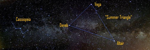
View larger. | Great Rift of Milky Way passes through the constellation Cassiopeia and the Summer Triangle.

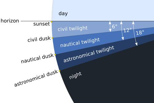
Summer Triangle as nature’s seasonal calendar. The Summer Triangle serves as a stellar calendar, marking the seasons. When the stars of the Summer Triangle light up the eastern twilight dusk in middle to late June, it’s a sure sign of the change of seasons, of spring giving way to summer. However, when the Summer Triangle is seen high in the south to overhead at dusk and early evening, the Summer Triangle’s change of position indicates that summer has ebbed into fall.

Bottom line: Coming to know the Summer Triangle, then seeing it again and again on summer nights, is a deep pleasure that adds to the enjoyment of this season.

EarthSky astronomy kits are perfect for beginners. Order today from the EarthSky store

Donate: Your support means the world to us

from EarthSky http://bit.ly/2X5m8j4

We in the Northern Hemisphere can see the Summer Triangle for part of the night at any time of the year. But seeing it in summer is the most fun! As suggested by its name, the Summer Triangle is most prominent during the summer season, for us at mid-northern latitudes. Seeing the Summer Triangle again and again on summer nights is a deep pleasure that adds to the enjoyment of this season. So, as dusk deepens into night on a warm June or July night, look eastward for this great star pattern … not a constellation, but instead an asterism made of three bright stars in three different constellations.

It’s difficult to convey the huge size of the Summer Triangle. At nightfall in northern summer, look for the brightest star in your eastern sky. That’s Vega, the brightest star in the constellation Lyra the Harp.

Look to the lower left of Vega for another bright star – Deneb, the brightest in the constellation Cygnus the Swan and the third brightest in the Summer Triangle. An outstretched hand at arm’s length approximates the distance from Vega to Deneb.

Look to the lower right of Vega to locate the Summer Triangle’s second brightest star. That’s Altair, the brightest star in the constellation Aquila the Eagle. A ruler held at arm’s length fills the gap between these two stars.

The Summer Triangle, as captured and composed by our friend Susan Gies Jensen in Odessa, Washington.

Summer Triangle as a road map to the Milky Way. If you’re lucky enough to be under a dark starry sky on a moonless night, you’ll see the great swath of stars known as the Milky Way passing in between the Summer Triangle stars Vega and Altair. The star Deneb bobs in the middle of this river of stars that passes through the Summer Triangle, and arcs across the sky. Although every star that you see with the unaided eye is actually a member of our Milky Way galaxy, often the term Milky Way refers to the cross-sectional view of the galactic disk, whereby innumerable far-off suns congregate into a cloudy trail of stars.

Once you master the Summer Triangle, you can always locate the Milky Way on a clear, dark night. How about making the most of a dark summer night to explore this band of stars – this starlit boulevard abounding with celestial delights? Use binoculars to reel in the gossamer beauty of it all, the haunting nebulae and star clusters of a midsummer night’s dream!

Some see the Summer Triangle as a great big “V” for vacation, with Altair marking the point of the “V.” In summer, the Summer Triangle appears in the east at nightfall, high overhead after midnight and in the west at dawn. All night long on a summer night, the stars of the Summer Triangle – as if school kids on vacation – waltz amidst the streetlights of the Milky Way galaxy.

Enjoying EarthSky so far? Sign up for our free daily newsletter today!

View larger. | Great Rift of Milky Way passes through the constellation Cassiopeia and the Summer Triangle.

Summer Triangle as nature’s seasonal calendar. The Summer Triangle serves as a stellar calendar, marking the seasons. When the stars of the Summer Triangle light up the eastern twilight dusk in middle to late June, it’s a sure sign of the change of seasons, of spring giving way to summer. However, when the Summer Triangle is seen high in the south to overhead at dusk and early evening, the Summer Triangle’s change of position indicates that summer has ebbed into fall.

Bottom line: Coming to know the Summer Triangle, then seeing it again and again on summer nights, is a deep pleasure that adds to the enjoyment of this season.

EarthSky astronomy kits are perfect for beginners. Order today from the EarthSky store

Donate: Your support means the world to us

from EarthSky http://bit.ly/2X5m8j4

The Trump EPA strategy to undo Clean Power Plan

This is a re-post from Yale Climate Connections

The Trump administration’s Environmental Protection Agency (EPA) on June 19 published its “Affordable Clean Energy” (ACE) rule to replace the Obama EPA’s Clean Power Plan (CPP).

The replacement plan is essentially the Trump administration’s attempt to adhere to the letter of the law mandating that carbon pollution be regulated, while requiring the smallest possible changes from the power utility industry. Preliminary research suggests that the ACE rule will barely reduce carbon emissions more than a scenario with no EPA policy whatsoever.

Current law says EPA must regulate carbon pollution

This story begins in 2003, when in response to a petition that the federal government regulate greenhouse gas emissions from motor vehicles, the George W. Bush EPA concluded that it did not have authority to do so under the Clean Air Act. Disagreeing with that determination, Democratic attorneys general of 12 states teamed up with several cities and environmental organizations to challenge that EPA action in court. The resulting litigation made it to the Supreme Court in 2007, and in the landmark Massachusetts v. Environmental Protection Agency ruling, the justices ruled 5-4 against the Bush administration and its EPA.

As a result, the agency was required to determine whether carbon dioxide and other greenhouse gases are air pollutants under the Clean Air Act, meaning that they “cause or contribute to air pollution which may reasonably be anticipated to endanger public health or welfare.”

In December 2009, EPA under President Obama completed its Endangerment Finding review of the scientific evidence and concluded that carbon pollution and other greenhouse gas emissions responsible for human-caused climate change clearly endanger public health and welfare. That determination led directly to the conclusion that the Clean Air Act requires that EPA regulate those pollutants, leading in turn to the Obama EPA’s CPP to strictly regulate utilities’ greenhouse gas emissions.

Emissions from motor vehicle tailpipes are addressed through corporate average fuel economy (CAFE) standards, which the Trump administration is also proposing to dramatically weaken in a battle with California and several other states, again all Democratically-controlled. To address pollution from power plants, the Obama EPA developed the CPP, which, if implemented, would have established national carbon emissions performance rates for coal and natural gas power plants while giving individual states some flexibility in finding ways to meet those standards.

Efforts to repeal and replace the Clean Power Plan

Opponents to the Obama EPA rulemaking wasted little time in launching numerous legal attacks against the CPP. The argument that had the most traction interpreted the Section 111(d) New Source Performance Standards elements of the Clean Air Act as giving EPA the authority to regulate only “within the fence line” of individual power plants. Under that interpretation, the agency would have exceeded its authority by regulating emissions from the power sector as a whole.

States, cities, and environmental organizations supportive of that CPP rule have argued that it is on solid legal ground with supporting precedents. But in 2016, the Supreme Court issued a stay to temporarily halt EPA enforcement of the plan pending lower court rulings on associated lawsuits. Barely two months into his term, President Trump signed an executive order calling on EPA under then-Administrator Scott Pruitt to review the CPP. Soon thereafter, the administration requested an indefinite suspension of the rule (a continued temporary suspension was granted).

Some persistent opponents of climate change rule-making efforts, like Trump EPA transition team members Myron Ebell and Steven Milloy and the fossil fuel-funded Competitive Enterprise Institute, have pressed the agency to challenge the Endangerment Finding. However, Pruitt disagreed with that strategy, fearing such an effort could backfire and be overruled by the courts in light of the compelling scientific basis for health concerns arising from climate change impacts. In fact, a February 2019 study published in the prestigious journal Science found that the scientific evidence supporting the Endangerment Finding has only strengthened over the past decade.

Instead, Pruitt and his successor at EPA, Andrew Wheeler, opted to replace the CPP with a more industry-friendly alternative, the “Affordable Clean Energy” rule, which is designed to help extend the lifetimes of expensive and heavily polluting coal-fired power plants. The June 19 release of the ACE rule now renders the CPP and associated lawsuits moot.

The new rule effectively implements the legal argument against the CPP by applying EPA regulations only to within the fence lines of individual power plants. Once implemented, it would provide states with various technological options that coal plants can install to help make them more efficient, thus potentially extending their lifespans. Because the new ACE rule establishes no numerical target for greenhouse gas emissions and allows states to consider factors like a plant’s “remaining useful life,” it could also allow state decisionmakers to conclude that no changes are needed at individual power plants.

The Trump administration has also argued that the CPP is no longer necessary. The plan’s goal was to cut carbon emissions from the power sector by 32 percent below 2005 levels by 2030; in 2017 they were already 28 percent below 2005 levels. However, U.S. power plant emissions rose slightly in 2018, a reflection of increased demand for natural gas. Critics of the new EPA rule caution that the trend toward cleaner electricity could certainly be slowed by fossil fuel-friendly policies such as the new ACE rule.

In addition, critics of ACE argue that since the power sector has been meeting the CPP targets so easily, EPA should be issuing more stringent targets and regulations to accelerate the clean energy transition, especially considering America’s current “critically insufficient” climate policies. A study published in Environmental Research Letters in April 2019 estimated that the ACE rule would lead to a negligible reduction in greenhouse gas emissions as compared to a “no policy” scenario. An analysis by the Natural Resources Defense Council (NDRC), a key national environmental organization, estimates that with the falling costs of clean energy, a stronger rule could cut power sector carbon pollution by 60 percent below 2005 levels by 2030, and do so at less cost than the initial estimated costs of the CPP. The NRDC study claimed billions of dollars in health benefits would result from cleaner air along with thousands of prevented premature deaths, consistent with EPA’s own analysis of ACE.

What comes next? Litigation and a big election

Numerous state attorneys general and environmental groups are certain to sue EPA over the new rule, arguing that it’s insufficient in scope to meet the agency’s regulatory obligations. Some legal experts have said they think the Trump administration would welcome a court challenge that could result in a Supreme Court ruling limiting EPA’s ability to regulate sector-wide greenhouse gas emissions from power plants.

The court challenges are expected to move forward slowly and incrementally, and if President Trump wins re-election for a second term in 2020, the Supreme Court will almost certainly be presented the case in the early 2020s. Those hoping for a supportive Supreme Court finding backing the new Trump rules appear hopeful – perhaps even confident – that the Court’s 2016 decision to temporarily halt the CPP is a sign that a majority of current justices are sympathetic to the Trump administration’s arguments.

With 2019 presidential campaign jockeying now well under way, most of the nearly two-dozen 2020 Democratic presidential hopefuls have said they plan to restore and/or strengthen the Obama-era CPP. But their succeeding with such an effort would require surviving an inevitable Supreme Court challenge. Congressional climate legislation – perhaps reflecting the general approach of the Green New Deal conceptually supported by most of the Democratic presidential candidates – could potentially negate the need for EPA power plant regulations. However, passage of comprehensive climate legislation would require that Democrats not only take control of the White House, but also win a majority in the Senate and maintain their majority in the House … and then also pass reforms to current Senate rules on filibusters.

None of those steps will come easily or, perhaps, come at all. So, in short, curbing carbon pollution is a major challenge under the current U.S. political system. Most conservative policymakers oppose climate legislation of the scale needed to address the problem, and the conservative-leaning Supreme Court – let alone a future Court that could have more Trump-nominated and Senate-confirmed justices – may be friendly to arguments against EPA’s authority to regulate the power sector under the existing Clean Air Act.

When it comes to U.S. action on climate change, uncertainty, for the time being, appears to be the only certainty.

from Skeptical Science http://bit.ly/2N8NIat

This is a re-post from Yale Climate Connections

The Trump administration’s Environmental Protection Agency (EPA) on June 19 published its “Affordable Clean Energy” (ACE) rule to replace the Obama EPA’s Clean Power Plan (CPP).

The replacement plan is essentially the Trump administration’s attempt to adhere to the letter of the law mandating that carbon pollution be regulated, while requiring the smallest possible changes from the power utility industry. Preliminary research suggests that the ACE rule will barely reduce carbon emissions more than a scenario with no EPA policy whatsoever.

Current law says EPA must regulate carbon pollution

This story begins in 2003, when in response to a petition that the federal government regulate greenhouse gas emissions from motor vehicles, the George W. Bush EPA concluded that it did not have authority to do so under the Clean Air Act. Disagreeing with that determination, Democratic attorneys general of 12 states teamed up with several cities and environmental organizations to challenge that EPA action in court. The resulting litigation made it to the Supreme Court in 2007, and in the landmark Massachusetts v. Environmental Protection Agency ruling, the justices ruled 5-4 against the Bush administration and its EPA.

As a result, the agency was required to determine whether carbon dioxide and other greenhouse gases are air pollutants under the Clean Air Act, meaning that they “cause or contribute to air pollution which may reasonably be anticipated to endanger public health or welfare.”

In December 2009, EPA under President Obama completed its Endangerment Finding review of the scientific evidence and concluded that carbon pollution and other greenhouse gas emissions responsible for human-caused climate change clearly endanger public health and welfare. That determination led directly to the conclusion that the Clean Air Act requires that EPA regulate those pollutants, leading in turn to the Obama EPA’s CPP to strictly regulate utilities’ greenhouse gas emissions.

Emissions from motor vehicle tailpipes are addressed through corporate average fuel economy (CAFE) standards, which the Trump administration is also proposing to dramatically weaken in a battle with California and several other states, again all Democratically-controlled. To address pollution from power plants, the Obama EPA developed the CPP, which, if implemented, would have established national carbon emissions performance rates for coal and natural gas power plants while giving individual states some flexibility in finding ways to meet those standards.

Efforts to repeal and replace the Clean Power Plan

Opponents to the Obama EPA rulemaking wasted little time in launching numerous legal attacks against the CPP. The argument that had the most traction interpreted the Section 111(d) New Source Performance Standards elements of the Clean Air Act as giving EPA the authority to regulate only “within the fence line” of individual power plants. Under that interpretation, the agency would have exceeded its authority by regulating emissions from the power sector as a whole.

States, cities, and environmental organizations supportive of that CPP rule have argued that it is on solid legal ground with supporting precedents. But in 2016, the Supreme Court issued a stay to temporarily halt EPA enforcement of the plan pending lower court rulings on associated lawsuits. Barely two months into his term, President Trump signed an executive order calling on EPA under then-Administrator Scott Pruitt to review the CPP. Soon thereafter, the administration requested an indefinite suspension of the rule (a continued temporary suspension was granted).

Some persistent opponents of climate change rule-making efforts, like Trump EPA transition team members Myron Ebell and Steven Milloy and the fossil fuel-funded Competitive Enterprise Institute, have pressed the agency to challenge the Endangerment Finding. However, Pruitt disagreed with that strategy, fearing such an effort could backfire and be overruled by the courts in light of the compelling scientific basis for health concerns arising from climate change impacts. In fact, a February 2019 study published in the prestigious journal Science found that the scientific evidence supporting the Endangerment Finding has only strengthened over the past decade.

Instead, Pruitt and his successor at EPA, Andrew Wheeler, opted to replace the CPP with a more industry-friendly alternative, the “Affordable Clean Energy” rule, which is designed to help extend the lifetimes of expensive and heavily polluting coal-fired power plants. The June 19 release of the ACE rule now renders the CPP and associated lawsuits moot.

The new rule effectively implements the legal argument against the CPP by applying EPA regulations only to within the fence lines of individual power plants. Once implemented, it would provide states with various technological options that coal plants can install to help make them more efficient, thus potentially extending their lifespans. Because the new ACE rule establishes no numerical target for greenhouse gas emissions and allows states to consider factors like a plant’s “remaining useful life,” it could also allow state decisionmakers to conclude that no changes are needed at individual power plants.

The Trump administration has also argued that the CPP is no longer necessary. The plan’s goal was to cut carbon emissions from the power sector by 32 percent below 2005 levels by 2030; in 2017 they were already 28 percent below 2005 levels. However, U.S. power plant emissions rose slightly in 2018, a reflection of increased demand for natural gas. Critics of the new EPA rule caution that the trend toward cleaner electricity could certainly be slowed by fossil fuel-friendly policies such as the new ACE rule.

In addition, critics of ACE argue that since the power sector has been meeting the CPP targets so easily, EPA should be issuing more stringent targets and regulations to accelerate the clean energy transition, especially considering America’s current “critically insufficient” climate policies. A study published in Environmental Research Letters in April 2019 estimated that the ACE rule would lead to a negligible reduction in greenhouse gas emissions as compared to a “no policy” scenario. An analysis by the Natural Resources Defense Council (NDRC), a key national environmental organization, estimates that with the falling costs of clean energy, a stronger rule could cut power sector carbon pollution by 60 percent below 2005 levels by 2030, and do so at less cost than the initial estimated costs of the CPP. The NRDC study claimed billions of dollars in health benefits would result from cleaner air along with thousands of prevented premature deaths, consistent with EPA’s own analysis of ACE.

What comes next? Litigation and a big election

Numerous state attorneys general and environmental groups are certain to sue EPA over the new rule, arguing that it’s insufficient in scope to meet the agency’s regulatory obligations. Some legal experts have said they think the Trump administration would welcome a court challenge that could result in a Supreme Court ruling limiting EPA’s ability to regulate sector-wide greenhouse gas emissions from power plants.

The court challenges are expected to move forward slowly and incrementally, and if President Trump wins re-election for a second term in 2020, the Supreme Court will almost certainly be presented the case in the early 2020s. Those hoping for a supportive Supreme Court finding backing the new Trump rules appear hopeful – perhaps even confident – that the Court’s 2016 decision to temporarily halt the CPP is a sign that a majority of current justices are sympathetic to the Trump administration’s arguments.

With 2019 presidential campaign jockeying now well under way, most of the nearly two-dozen 2020 Democratic presidential hopefuls have said they plan to restore and/or strengthen the Obama-era CPP. But their succeeding with such an effort would require surviving an inevitable Supreme Court challenge. Congressional climate legislation – perhaps reflecting the general approach of the Green New Deal conceptually supported by most of the Democratic presidential candidates – could potentially negate the need for EPA power plant regulations. However, passage of comprehensive climate legislation would require that Democrats not only take control of the White House, but also win a majority in the Senate and maintain their majority in the House … and then also pass reforms to current Senate rules on filibusters.

None of those steps will come easily or, perhaps, come at all. So, in short, curbing carbon pollution is a major challenge under the current U.S. political system. Most conservative policymakers oppose climate legislation of the scale needed to address the problem, and the conservative-leaning Supreme Court – let alone a future Court that could have more Trump-nominated and Senate-confirmed justices – may be friendly to arguments against EPA’s authority to regulate the power sector under the existing Clean Air Act.

When it comes to U.S. action on climate change, uncertainty, for the time being, appears to be the only certainty.

from Skeptical Science http://bit.ly/2N8NIat

Unusually high methane levels detected on Mars

This image was taken by the Curiosity Mars rover’s camera on June 18, 2019. Image via NASA/JPL-Caltech.

In a statement released yesterday (June 23, 2919) NASA reported that last week, its Curiosity Mars rover measured the largest yet level of methane in the Martian atmosphere – about 21 parts per billion units by volume (ppbv) – since landing on the planet in August 2012.

One ppbv means that if you take a volume of air on Mars, one billionth of the volume of air is methane.

It’s exciting, NASA said, because here on Earth, microbial life is an important source of the methane gas in our air, although methane can also be created through interactions between rocks and water. As for how the methane was produced on Mars, scientists aren’t sure. Curiosity doesn’t have instruments that can definitively pinpoint the methane’s source.

NASA’s Curiosity Mars rover took this selfie on May 12, 2019. Image via NASA/JPL-Caltech/MSSS

Mission scientist Paul Mahaffy, of NASA’s Goddard Spaceflight Center, said:

With our current measurements, we have no way of telling if the methane source is biology or geology, or even ancient or modern.

The Curiosity team has detected methane many times over the course of the mission. Previous papers have documented how background levels of the gas seem to rise and fall seasonally, and noted sudden spikes of methane.

But the science team knows very little about how long these transient plumes last or why they’re different from the seasonal patterns. The new measurement also deepens the mystery of why the European Space Agency’s ExoMars Space Gas Orbiter, a probe sent to Mars to look for methane, has so far found no traces of the gas. Read more about the strange case of Mars’ disappearing methane.

NASA scientists plan further experiments for to gather more information on what might be a transient plume. Whatever they find — even if it’s an absence of methane — will add context to the recent measurement.

Via NASA

Bottom line: NASAs Mars Curiosity rover detected its largest-yet spike of methane.

from EarthSky http://bit.ly/2KC4QTK

This image was taken by the Curiosity Mars rover’s camera on June 18, 2019. Image via NASA/JPL-Caltech.

In a statement released yesterday (June 23, 2919) NASA reported that last week, its Curiosity Mars rover measured the largest yet level of methane in the Martian atmosphere – about 21 parts per billion units by volume (ppbv) – since landing on the planet in August 2012.

One ppbv means that if you take a volume of air on Mars, one billionth of the volume of air is methane.

It’s exciting, NASA said, because here on Earth, microbial life is an important source of the methane gas in our air, although methane can also be created through interactions between rocks and water. As for how the methane was produced on Mars, scientists aren’t sure. Curiosity doesn’t have instruments that can definitively pinpoint the methane’s source.

NASA’s Curiosity Mars rover took this selfie on May 12, 2019. Image via NASA/JPL-Caltech/MSSS

Mission scientist Paul Mahaffy, of NASA’s Goddard Spaceflight Center, said:

With our current measurements, we have no way of telling if the methane source is biology or geology, or even ancient or modern.

The Curiosity team has detected methane many times over the course of the mission. Previous papers have documented how background levels of the gas seem to rise and fall seasonally, and noted sudden spikes of methane.

But the science team knows very little about how long these transient plumes last or why they’re different from the seasonal patterns. The new measurement also deepens the mystery of why the European Space Agency’s ExoMars Space Gas Orbiter, a probe sent to Mars to look for methane, has so far found no traces of the gas. Read more about the strange case of Mars’ disappearing methane.

NASA scientists plan further experiments for to gather more information on what might be a transient plume. Whatever they find — even if it’s an absence of methane — will add context to the recent measurement.

Via NASA

Bottom line: NASAs Mars Curiosity rover detected its largest-yet spike of methane.

from EarthSky http://bit.ly/2KC4QTK

Table salt compound spotted on Jupiter’s moon Europa

Natural color (left) and enhanced color (right) views of Europa from the Galileo mission in June 1997. The yellowish regions are now known to be caused by sodium chloride, also known as table salt, the principal component of sea salt. Image via NASA JPL-Caltech/University of Arizona.

Europa’s subsurface ocean might be even more similar to Earth’s oceans than previously realized. NASA said on June 12, 2019, that a new study reveals evidence of sodium chloride – a major component of table salt and sea salt – on the icy surface of this large moon of Jupiter. If, as thought, the salt originates from Europa’s ocean, hidden beneath its icy crust, that would mean Europa’s ocean water is very similar to that in oceans on Earth. That, of course, would have obvious implications for the possibility of life on this fascinating little world.

The intriguing new peer-reviewed findings were published in the journal Science Advances on June 12, 2019.

The fact that sodium chloride is also a principal component of sea salt is particularly fascinating. Its discovery on Europa supports previous suggestions that this moon’s ocean is chemically very similar to Earth’s oceans.

Even though Europa’s ocean isn’t on its surface – but instead below its surface ice, surrounded by the icy shell of Europa’s crust – traces of minerals can be found on the little moon’s surface. The surface salt is thought to be due to upwelling through cracks and possibly geysers. Previous studies of the surface, including from NASA’s Voyager and Galileo spacecraft, had focused on infrared spectroscopy, since it is ideal for detecting the kinds of molecules that scientists are usually looking for. According to Mike Brown, an astronomer at Caltech:

People have traditionally assumed that all of the interesting spectroscopy is in the infrared on planetary surfaces, because that’s where most of the molecules that scientists are looking for have their fundamental features.

In a test lab at the Jet Propulsion Laboratory, table salt – sodium chloride – turned yellow when subjected to similar radiation conditions as those on the surface of Europa. Image via NASA JPL-Caltech.

These types of chlorides can’t be seen with infrared spectroscopy, however, as Caltech student Samantha Trumbo explained:

No one has taken visible-wavelength spectra of Europa before that had this sort of spatial and spectral resolution. The Galileo spacecraft didn’t have a visible spectrometer. It just had a near-infrared spectrometer, and in the near-infrared, chlorides are featureless.

But when viewed in visible-wavelength spectroscopy, the sodium chloride signature popped out.

Previously, it was thought that magnesium sulfates had been found on the surface, but when additional higher quality observations were conducted with the W. M. Keck Observatory in Hawaii, there was no sign of them. The data pointed more towards sodium chlorides instead, and those don’t show up in infrared. As Brown also noted:

We thought that we might be seeing sodium chlorides, but they are essentially featureless in an infrared spectrum.

Europa’s cracked icy surface as seen by NASA’s Galileo spacecraft in the late 1990s. Yellowish regions on the moon’s surface have now been confirmed to be irradiated sodium chloride, aka table salt. Image via NASA/JPL-Caltech/SETI Institute.

Map showing the areas where the sodium chloride salts are found on Europa’s surface. The highest concentrations are in the Tara Regio region. Image via NASA/JPL/Björn Jónsson/Steve Albers/Science Advances.

Proving that the salts were sodium chloride still required a bit more work, however. Samples of similar ocean salts were tested on Earth by Kevin Hand at JPL. He subjected them to similar radiation conditions found on Europa’s airless surface. He found that they changed colors in a manner very similar to what is actually seen on Europa itself. The sodium chloride turned a shade of yellow similar to that seen in a geologically young area of Europa known as Tara Regio. According to Hand:

Sodium chloride is a bit like invisible ink on Europa’s surface. Before irradiation you can’t tell it’s there, but after irradiation the color jumps right out at you.

The research team then studied Europa’s surface with the Hubble Space Telescope, and found a distinct absorption signature in the visible spectrum at 450 nanometers. This matched exactly the irradiated form of sodium chloride, confirming that the yellow color of Tara Regio showed the presence of the salt on the surface. So why wasn’t this found already? As Brown said:

We’ve had the capacity to do this analysis with the Hubble Space Telescope for the past 20 years. It’s just that nobody thought to look.

There’s still one caveat – the sodium chloride might be evidence of different types of materials stratified – formed in layers – in the moon’s icy shell, rather than originating from the ocean. The finding, however, is enough to warrant a reevaluation of the geochemistry of Europa as a whole. If indeed the sodium chloride does originate from the ocean, it would be evidence that the ocean floor is still hydrothermally active. According to Trumbo:

Magnesium sulfate would simply have leached into the ocean from rocks on the ocean floor, but sodium chloride may indicate the ocean floor is hydrothermally active. That would mean Europa is a more geologically interesting planetary body than previously believed.

Illustration of Europa’s outer ice crust. It’s thought that water from the ocean below can reach the surface through cracks or volcanic vents. This is the salts are most likely deposited onto the surface. Image via NASA/JPL-Caltech/Geology.com.

If the ocean floor on Europa does have active hydrothermal vents like in Earth’s oceans, that would boost the chances for some kind of life to exist there. On Earth, such “hotspots” in the deep oceans are oases for living organisms.

Saturn’s ocean moon Enceladus is also now thought to have hydrothermal vents on its ocean bottom, based on data from NASA’s Cassini mission, which ended in late 2017. Scientists now know that Enceladus’ ocean contains salts and a variety of organic molecules, thanks to Cassini being able to fly through and directly sample some of the huge water vapor plumes that erupt from cracks in the moon’s icy surface and originate from the ocean deep below. Cassini couldn’t detect life itself, even if it was there, but future missions will search for that evidence at both Enceladus and Europa.

Bottom line: The discovery of sodium chloride salts on Europa provides compelling evidence that the moon’s subsurface ocean is very similar to Earth’s oceans, increasing the chances for life.

Source: Sodium chloride on the surface of Europa

Via NASA

from EarthSky http://bit.ly/2Fuf6tf

Natural color (left) and enhanced color (right) views of Europa from the Galileo mission in June 1997. The yellowish regions are now known to be caused by sodium chloride, also known as table salt, the principal component of sea salt. Image via NASA JPL-Caltech/University of Arizona.

Europa’s subsurface ocean might be even more similar to Earth’s oceans than previously realized. NASA said on June 12, 2019, that a new study reveals evidence of sodium chloride – a major component of table salt and sea salt – on the icy surface of this large moon of Jupiter. If, as thought, the salt originates from Europa’s ocean, hidden beneath its icy crust, that would mean Europa’s ocean water is very similar to that in oceans on Earth. That, of course, would have obvious implications for the possibility of life on this fascinating little world.

The intriguing new peer-reviewed findings were published in the journal Science Advances on June 12, 2019.

The fact that sodium chloride is also a principal component of sea salt is particularly fascinating. Its discovery on Europa supports previous suggestions that this moon’s ocean is chemically very similar to Earth’s oceans.

Even though Europa’s ocean isn’t on its surface – but instead below its surface ice, surrounded by the icy shell of Europa’s crust – traces of minerals can be found on the little moon’s surface. The surface salt is thought to be due to upwelling through cracks and possibly geysers. Previous studies of the surface, including from NASA’s Voyager and Galileo spacecraft, had focused on infrared spectroscopy, since it is ideal for detecting the kinds of molecules that scientists are usually looking for. According to Mike Brown, an astronomer at Caltech:

People have traditionally assumed that all of the interesting spectroscopy is in the infrared on planetary surfaces, because that’s where most of the molecules that scientists are looking for have their fundamental features.

In a test lab at the Jet Propulsion Laboratory, table salt – sodium chloride – turned yellow when subjected to similar radiation conditions as those on the surface of Europa. Image via NASA JPL-Caltech.

These types of chlorides can’t be seen with infrared spectroscopy, however, as Caltech student Samantha Trumbo explained:

No one has taken visible-wavelength spectra of Europa before that had this sort of spatial and spectral resolution. The Galileo spacecraft didn’t have a visible spectrometer. It just had a near-infrared spectrometer, and in the near-infrared, chlorides are featureless.

But when viewed in visible-wavelength spectroscopy, the sodium chloride signature popped out.

Previously, it was thought that magnesium sulfates had been found on the surface, but when additional higher quality observations were conducted with the W. M. Keck Observatory in Hawaii, there was no sign of them. The data pointed more towards sodium chlorides instead, and those don’t show up in infrared. As Brown also noted:

We thought that we might be seeing sodium chlorides, but they are essentially featureless in an infrared spectrum.

Europa’s cracked icy surface as seen by NASA’s Galileo spacecraft in the late 1990s. Yellowish regions on the moon’s surface have now been confirmed to be irradiated sodium chloride, aka table salt. Image via NASA/JPL-Caltech/SETI Institute.

Map showing the areas where the sodium chloride salts are found on Europa’s surface. The highest concentrations are in the Tara Regio region. Image via NASA/JPL/Björn Jónsson/Steve Albers/Science Advances.

Proving that the salts were sodium chloride still required a bit more work, however. Samples of similar ocean salts were tested on Earth by Kevin Hand at JPL. He subjected them to similar radiation conditions found on Europa’s airless surface. He found that they changed colors in a manner very similar to what is actually seen on Europa itself. The sodium chloride turned a shade of yellow similar to that seen in a geologically young area of Europa known as Tara Regio. According to Hand:

Sodium chloride is a bit like invisible ink on Europa’s surface. Before irradiation you can’t tell it’s there, but after irradiation the color jumps right out at you.

The research team then studied Europa’s surface with the Hubble Space Telescope, and found a distinct absorption signature in the visible spectrum at 450 nanometers. This matched exactly the irradiated form of sodium chloride, confirming that the yellow color of Tara Regio showed the presence of the salt on the surface. So why wasn’t this found already? As Brown said:

We’ve had the capacity to do this analysis with the Hubble Space Telescope for the past 20 years. It’s just that nobody thought to look.

There’s still one caveat – the sodium chloride might be evidence of different types of materials stratified – formed in layers – in the moon’s icy shell, rather than originating from the ocean. The finding, however, is enough to warrant a reevaluation of the geochemistry of Europa as a whole. If indeed the sodium chloride does originate from the ocean, it would be evidence that the ocean floor is still hydrothermally active. According to Trumbo:

Magnesium sulfate would simply have leached into the ocean from rocks on the ocean floor, but sodium chloride may indicate the ocean floor is hydrothermally active. That would mean Europa is a more geologically interesting planetary body than previously believed.

Illustration of Europa’s outer ice crust. It’s thought that water from the ocean below can reach the surface through cracks or volcanic vents. This is the salts are most likely deposited onto the surface. Image via NASA/JPL-Caltech/Geology.com.

If the ocean floor on Europa does have active hydrothermal vents like in Earth’s oceans, that would boost the chances for some kind of life to exist there. On Earth, such “hotspots” in the deep oceans are oases for living organisms.

Saturn’s ocean moon Enceladus is also now thought to have hydrothermal vents on its ocean bottom, based on data from NASA’s Cassini mission, which ended in late 2017. Scientists now know that Enceladus’ ocean contains salts and a variety of organic molecules, thanks to Cassini being able to fly through and directly sample some of the huge water vapor plumes that erupt from cracks in the moon’s icy surface and originate from the ocean deep below. Cassini couldn’t detect life itself, even if it was there, but future missions will search for that evidence at both Enceladus and Europa.

Bottom line: The discovery of sodium chloride salts on Europa provides compelling evidence that the moon’s subsurface ocean is very similar to Earth’s oceans, increasing the chances for life.

Source: Sodium chloride on the surface of Europa

Via NASA

from EarthSky http://bit.ly/2Fuf6tf

Screams contain a 'calling card' for the vocalizer's identity

"Our findings add to our understanding of how screams are evolutionarily important," says Emory psychologist Harold Gouzoules, senior author of the paper.

By Carol Clark

Human screams convey a level of individual identity that may help explain their evolutionary origins, finds a study by scientists at Emory University.

PeerJ published the research, showing that listeners can correctly identify whether pairs of screams were produced by the same person or two different people — a critical prerequisite to individual recognition.

“Our findings add to our understanding of how screams are evolutionarily important,” says Harold Gouzoules, senior author of the paper and an Emory professor of psychology. “The ability to identify who is screaming is likely an adaptive mechanism. The idea is that you wouldn’t respond equally to just anyone’s scream. You would likely respond more urgently to a scream from your child, or from someone else important to you.”

Jonathan Engelberg is first author of the paper and Jay Schwartz is a co-author. They are both Emory PhD candidates in Gouzoules’ Bioacoustics Lab.

The ability to recognize individuals by distinctive cues or signals is essential to the organization of social behavior, the authors note, and humans are adept at making identity-related judgements based on speech — even when the speech is heavily altered. Less is known, however, about identity cues in nonlinguistic vocalizations, such as screams.

Gouzoules first began researching monkey screams in 1980, before becoming one of the few scientists studying human screams about 10 years ago.

“The origin of screams was likely to startle a predator and make it jump, perhaps allowing the prey a small chance to escape,” Gouzoules says. “That’s very different from calling out for help.”

He theorizes that as some species became more social, including monkeys and other primates, screams became a way to recruit help from relatives and friends when someone got into trouble.

Previous research by Gouzoules and others suggests that non-human primates are able to identify whether a scream is coming from an individual that is important to them. Some researchers, however, have disputed the evidence, arguing that the chaotic and inconsistent nature of screams does not make them likely conduits for individual recognition.

Gouzoules wanted to test whether humans could determine if two fairly similar screams were made by the same person or a different person. His Bioacoustics Lab has amassed an impressive library of high-intensity, visceral sounds — from TV and movie performances to the screams of non-actors reacting to actual events on YouTube videos.

For the PeerJ paper, the lab ran experiments that included 104 participants. The participants listened to audio files of pairs of screams on a computer, without any visual cues for context. Each pair was presented two seconds apart and participants were asked to determine if the screams came from the same person or a different person.

In some trials, the two screams came from two different callers, but were matched by age, gender and the context of the scream. In other trials, the screams came from the same caller but were two different screams matched for context. And in a third trial, the stimulus pairs consisted of a scream and a slightly modified version of itself, to make it longer or shorter than the original.

For all three of the experiments, most of the participants were able to correctly judge most of the time whether the screams were from the same person or not.

“Our results provide empirical evidence that screams carry enough information for listeners to discriminate between different callers,” Gouzoules says. “Although screams may not be acoustically ideal for signaling a caller’s identity, natural selection appears to have adequately shaped them so they are good enough to do the job.”

The PeerJ paper is part of an extensive program of research into screams by Gouzoules. In previous work, his lab has found that listeners cannot distinguish acted screams from naturally occurring screams.

In upcoming papers, he is zeroing in on how people determine whether they are hearing a scream or some other vocalization and how they perceive the emotional context of a scream — judging whether it’s due to happiness, anger, fear or pain.

Photo: Getty Images

Related:
The psychology of screams

from eScienceCommons http://bit.ly/2WZApZJ

"Our findings add to our understanding of how screams are evolutionarily important," says Emory psychologist Harold Gouzoules, senior author of the paper.

By Carol Clark

Human screams convey a level of individual identity that may help explain their evolutionary origins, finds a study by scientists at Emory University.

PeerJ published the research, showing that listeners can correctly identify whether pairs of screams were produced by the same person or two different people — a critical prerequisite to individual recognition.

“Our findings add to our understanding of how screams are evolutionarily important,” says Harold Gouzoules, senior author of the paper and an Emory professor of psychology. “The ability to identify who is screaming is likely an adaptive mechanism. The idea is that you wouldn’t respond equally to just anyone’s scream. You would likely respond more urgently to a scream from your child, or from someone else important to you.”

Jonathan Engelberg is first author of the paper and Jay Schwartz is a co-author. They are both Emory PhD candidates in Gouzoules’ Bioacoustics Lab.

The ability to recognize individuals by distinctive cues or signals is essential to the organization of social behavior, the authors note, and humans are adept at making identity-related judgements based on speech — even when the speech is heavily altered. Less is known, however, about identity cues in nonlinguistic vocalizations, such as screams.

Gouzoules first began researching monkey screams in 1980, before becoming one of the few scientists studying human screams about 10 years ago.

“The origin of screams was likely to startle a predator and make it jump, perhaps allowing the prey a small chance to escape,” Gouzoules says. “That’s very different from calling out for help.”

He theorizes that as some species became more social, including monkeys and other primates, screams became a way to recruit help from relatives and friends when someone got into trouble.

Previous research by Gouzoules and others suggests that non-human primates are able to identify whether a scream is coming from an individual that is important to them. Some researchers, however, have disputed the evidence, arguing that the chaotic and inconsistent nature of screams does not make them likely conduits for individual recognition.

Gouzoules wanted to test whether humans could determine if two fairly similar screams were made by the same person or a different person. His Bioacoustics Lab has amassed an impressive library of high-intensity, visceral sounds — from TV and movie performances to the screams of non-actors reacting to actual events on YouTube videos.

For the PeerJ paper, the lab ran experiments that included 104 participants. The participants listened to audio files of pairs of screams on a computer, without any visual cues for context. Each pair was presented two seconds apart and participants were asked to determine if the screams came from the same person or a different person.

In some trials, the two screams came from two different callers, but were matched by age, gender and the context of the scream. In other trials, the screams came from the same caller but were two different screams matched for context. And in a third trial, the stimulus pairs consisted of a scream and a slightly modified version of itself, to make it longer or shorter than the original.

For all three of the experiments, most of the participants were able to correctly judge most of the time whether the screams were from the same person or not.

“Our results provide empirical evidence that screams carry enough information for listeners to discriminate between different callers,” Gouzoules says. “Although screams may not be acoustically ideal for signaling a caller’s identity, natural selection appears to have adequately shaped them so they are good enough to do the job.”

The PeerJ paper is part of an extensive program of research into screams by Gouzoules. In previous work, his lab has found that listeners cannot distinguish acted screams from naturally occurring screams.

In upcoming papers, he is zeroing in on how people determine whether they are hearing a scream or some other vocalization and how they perceive the emotional context of a scream — judging whether it’s due to happiness, anger, fear or pain.

Photo: Getty Images

Related:
The psychology of screams

from eScienceCommons http://bit.ly/2WZApZJ

Science Snaps: seeing the effects of proteins we know nothing about

Anh Hoang Le, a PhD student at the Cancer Research UK Beatson Institute in Glasgow, studies two proteins that we know curiously little about: CYRI-A and CYRI-B.

“We have some hints that they might be involved in cancer, and it’s my teams’ job to find out if it’s true.”

Le has been growing batches of cancer cells in the lab that have one key difference: some can produce the CYRI proteins, while others can’t. He then looks for differences between the cells using tools similar to microscopes.

And so far, the most striking of these has been changes in cell shape, which can have an important effect on how the cell behaves.

“I have four different stains on these cells so you can see four different things. The nucleus is the round blue balls in the middle of each cell, which contains DNA. The cytoskeleton, which essentially is the skeleton of the cell, is in magenta. The yellow is a protein called ArpC2, and the green is a protein called integrin,” he explains.

The molecules aren’t usually those colours. Le sticks a different fluorescent dye to each molecule to make them glow. It’s a standard technique in cell biology if you want to look at things inside a cell. And it produces some beautiful images while you’re at it.

Supporting roles – integrin and ArpC2

The image on the left is a regular cancer cell. Whereas the cell on the right is a cancer cell that has had the proteins CYRI-A and CYRI-B removed. The cell’s shape has changed dramatically and a protein called integrin (green) changes location inside the cell. A molecule called ArpC2 (yellow) becomes concentrated around the edges of the cell, meaning the cell may be more likely to move. Image credit: Anh Hoang Le, CRUK Beatson Institute.

Integrin, in green, has multiple jobs. But one of its most important roles is sticking the cell to its surroundings, like an anchor. It’s known to be key in deciding the shape of the cell. And it’s been linked to the spread of cancer cells around the body.

In an earlier experiment, Le found that when he removed the CYRI proteins from cells, they became stickier. But they also moved faster than cells with the CYRI proteins. As integrin is known to be involved in both these processes, Le decided to look at the location and amount of integrin inside the cells.

The image above shows a regular cancer cell on the left, and one that been engineered so it doesn’t produce the CYRI proteins, on the right.

“When I removed the proteins from the cell, it changes shape. And you can see that when they are present, the integrin is very spread inside the cell. But without, you can suddenly see all of those green stripes that align with the cell. So without the CYRI proteins, integrin is more prominent and is perhaps helping the cell to move.”

Another protein called ArpC2, marked yellow in the image, is also important in cell movement. The protein collects at the edges of the cell when it wants to move, which is what happens in cells without the CYRI proteins.

Overall, Le thinks CYRI-A and CYRI-B may be changing the distribution of integrin and ArpC2 inside cells, which leads to the change in shape. And this could trigger cancer cells to move.

Shaping up nicely

Again, The image on the left is a regular cancer cell. The cell on the right has had the CYRI proteins removed. The cell has changed shape and integrin (green) is aligned throughout the cell, while ArpC2 (yellow) are concentrated around the edge of the cell. Image Credit: Anh Hoang Le, CRUK Beatson Institute.

The shape of a cell is important because it indicates what the cell may be likely to do, whether that be multiply, move or die.

“The cell with the proteins has very spiky protrusions,” says Le. “Those spikes are called filopodia, which we think are for the cell to sense its environment.”

Cancer cells without the CYRI proteins have less obvious protrusions. In the right-hand image above, they’re the small bumps around the edge of the cell. “We call that lamellipodia, which we think is more for a cell to ‘crawl’,” says Le.

Le’s lab research suggests that if cancer cells lose the ability to make the CYRI proteins they may be more likely to move, which could be linked to cancer spread (metastasis). But it’s early days.

“There is a lot of debate,” warns Le. “So it is difficult to firmly say that if you have more lamellipodia the cell is going to metastasise, because inside the actual cancer there are a lot of interactions and factors that we don’t have enough knowledge about yet.”

According to Le, which structures are important for cancer to progress may actually differ depending on the cancer type.

For now, Le’s work is helping uncover the roles of these mysterious proteins in cancer. And he’s produced some great images along the way.

“My favourite? I think it’s the ‘fan-shaped’ one. Because, compared to the spiky one, it gives you a striking look at how different the cell shape is when the proteins are not there.”

Ethan

Reference

Fort et. al. (2018). Fam49/CYRI interacts with Rac1 and locally suppresses protrusions. Nature. DOI: 10.1038/s41556-018-0198-9

from Cancer Research UK – Science blog http://bit.ly/2IGcESy

Anh Hoang Le, a PhD student at the Cancer Research UK Beatson Institute in Glasgow, studies two proteins that we know curiously little about: CYRI-A and CYRI-B.

“We have some hints that they might be involved in cancer, and it’s my teams’ job to find out if it’s true.”

Le has been growing batches of cancer cells in the lab that have one key difference: some can produce the CYRI proteins, while others can’t. He then looks for differences between the cells using tools similar to microscopes.

And so far, the most striking of these has been changes in cell shape, which can have an important effect on how the cell behaves.

“I have four different stains on these cells so you can see four different things. The nucleus is the round blue balls in the middle of each cell, which contains DNA. The cytoskeleton, which essentially is the skeleton of the cell, is in magenta. The yellow is a protein called ArpC2, and the green is a protein called integrin,” he explains.

The molecules aren’t usually those colours. Le sticks a different fluorescent dye to each molecule to make them glow. It’s a standard technique in cell biology if you want to look at things inside a cell. And it produces some beautiful images while you’re at it.

Supporting roles – integrin and ArpC2

The image on the left is a regular cancer cell. Whereas the cell on the right is a cancer cell that has had the proteins CYRI-A and CYRI-B removed. The cell’s shape has changed dramatically and a protein called integrin (green) changes location inside the cell. A molecule called ArpC2 (yellow) becomes concentrated around the edges of the cell, meaning the cell may be more likely to move. Image credit: Anh Hoang Le, CRUK Beatson Institute.

Integrin, in green, has multiple jobs. But one of its most important roles is sticking the cell to its surroundings, like an anchor. It’s known to be key in deciding the shape of the cell. And it’s been linked to the spread of cancer cells around the body.

In an earlier experiment, Le found that when he removed the CYRI proteins from cells, they became stickier. But they also moved faster than cells with the CYRI proteins. As integrin is known to be involved in both these processes, Le decided to look at the location and amount of integrin inside the cells.

The image above shows a regular cancer cell on the left, and one that been engineered so it doesn’t produce the CYRI proteins, on the right.

“When I removed the proteins from the cell, it changes shape. And you can see that when they are present, the integrin is very spread inside the cell. But without, you can suddenly see all of those green stripes that align with the cell. So without the CYRI proteins, integrin is more prominent and is perhaps helping the cell to move.”

Another protein called ArpC2, marked yellow in the image, is also important in cell movement. The protein collects at the edges of the cell when it wants to move, which is what happens in cells without the CYRI proteins.

Overall, Le thinks CYRI-A and CYRI-B may be changing the distribution of integrin and ArpC2 inside cells, which leads to the change in shape. And this could trigger cancer cells to move.

Shaping up nicely

Again, The image on the left is a regular cancer cell. The cell on the right has had the CYRI proteins removed. The cell has changed shape and integrin (green) is aligned throughout the cell, while ArpC2 (yellow) are concentrated around the edge of the cell. Image Credit: Anh Hoang Le, CRUK Beatson Institute.

The shape of a cell is important because it indicates what the cell may be likely to do, whether that be multiply, move or die.

“The cell with the proteins has very spiky protrusions,” says Le. “Those spikes are called filopodia, which we think are for the cell to sense its environment.”

Cancer cells without the CYRI proteins have less obvious protrusions. In the right-hand image above, they’re the small bumps around the edge of the cell. “We call that lamellipodia, which we think is more for a cell to ‘crawl’,” says Le.

Le’s lab research suggests that if cancer cells lose the ability to make the CYRI proteins they may be more likely to move, which could be linked to cancer spread (metastasis). But it’s early days.

“There is a lot of debate,” warns Le. “So it is difficult to firmly say that if you have more lamellipodia the cell is going to metastasise, because inside the actual cancer there are a lot of interactions and factors that we don’t have enough knowledge about yet.”

According to Le, which structures are important for cancer to progress may actually differ depending on the cancer type.

For now, Le’s work is helping uncover the roles of these mysterious proteins in cancer. And he’s produced some great images along the way.

“My favourite? I think it’s the ‘fan-shaped’ one. Because, compared to the spiky one, it gives you a striking look at how different the cell shape is when the proteins are not there.”

Ethan

Reference

Fort et. al. (2018). Fam49/CYRI interacts with Rac1 and locally suppresses protrusions. Nature. DOI: 10.1038/s41556-018-0198-9

from Cancer Research UK – Science blog http://bit.ly/2IGcESy

6 amazing facts about ants

Image via Wikipedia.

By Charlie Durant, University of Leicester; Max John, University of Leicester, and Rob Hammond, University of Leicester

Have you have seen ants this year? In Britain, they were probably black garden ants, known as Lasius niger – Europe’s most common ant. One of somewhere between 12,000 and 20,000 species, they are the scourge of gardeners – but also fascinating.

The small, black, wingless workers run around the pavements, crawl up your plants tending aphids or collect tasty morsels from your kitchen. And the flying ants that occasionally appear on a warm summer’s evening are actually the reproductive siblings of these non-winged workers. Here’s what else you need to know:

1. Most ants you see are female

Ants have a caste system, where responsibilities are divided. The queen is the founder of the colony, and her role is to lay eggs. Worker ants are all female, and this sisterhood is responsible for the harmonious operation of the colony.

Their tasks range from caring for the queen and the young, foraging, policing conflicts in the colony, and waste disposal. Workers will most likely never have their own offspring. The vast majority of eggs develop as workers, but once the colony is ready the queen produces the next generation of reproductives which will go on to start own colonies.

A female ant’s fate to become a worker or queen is mainly determined by diet, not genetics. Any female ant larva can become the queen – those that do receive diets richer in protein. The other larvae receive less protein, which causes them to develop as workers.

2. Male ants are pretty much just flying sperm

Male ants have a mother but no father.

Unlike humans, with X and Y chromosomes, an ant’s sex is determined by the number of genome copies it possesses. Male ants develop from unfertilized eggs so receive no genome from a father. This means that male ants don’t have a father and cannot have sons, but they do have grandfathers and can have grandsons. Female ants, in comparison, develop from fertilized eggs and have two genome copies – one from their father and one from their mother.

Male ants function like flying sperm. Only having one genome copy means every one of their sperm is genetically identical to themselves. And their job is over quickly, dying soon after mating, although their sperm live on, perhaps for years. Essentially, their only job is to reproduce.

Let them eat cake. Image via Shutterstock.

3. After sex, queens don’t eat for weeks

When the conditions are warm and humid, the winged virgin queens and males leave their nests in search of mates. This is the behavior seen on “flying ant day”. In L. niger, mating takes place on the wing, often hundreds of meters [yards] up (hence the need for good weather). Afterwards, queens drop to the ground and shed their wings, while males quickly die. Mated queens choose a nest site and burrow into the soil, made softer from recent rain.

Once underground, the queens will not eat for weeks – until they have produced their own daughter workers. They use energy from their fat stores and redundant flight muscles to lay their first batch of eggs, which they fertilize using sperm stored from their nuptial flight. It is the same stock of sperm acquired from long dead males that allows a queen to continue laying fertilized eggs for her entire life. Queens never mate again.

4. Home-making the ant way is about cooperation, death and slavery

Sometimes two L. niger queens unite to found a nest. This initially cooperative association – which increases the chance of establishing a colony – dissolves once new adult workers emerge and then the queens fight to the death. More sinister still, L. niger colonies sometimes steal brood from their neighbors, putting them to work as slaves.

Slave-making has evolved in a number of ant species, but they also display cooperation at extraordinary levels. An extreme example of this is a “supercolony” of Argentine ants (Linepithema humile) which extends over 3,700 miles (6,000 km) of European coastline from Italy to northwest Spain, and is composed of literally billions of workers from millions of cooperating nests.

5. Queen ants can live for decades, males for a week

After establishing her colony, the queen’s work is not done and she has many years of egg-laying ahead of her. In the laboratory, L. niger queens have lived for nearly 30 years. Workers live for about a year, males little more than a week (although their sperm live longer). These extraordinary differences in longevity are purely due to the way their genes are switched on and off.

6. Ants can help humans and the environment

Ants have a major influence in ecosystems worldwide and their roles are diverse. While some ants are considered pests, others act as biological-control agents. Ants benefit ecosystems by dispersing seeds, pollinating plants and improving the quality of soil. Ants might also benefit our health, as a potential source of new medicines such as antibiotics.

So when you next see an ant, before you think to kill her, consider how fascinating she really is.

Charlie Durant, Ph.D. candidate, Department of Genetics and Genome Biology, University of Leicester; Max John, Ph.D. candidate, Department of Genetics and Genome Biology, University of Leicester, and Rob Hammond, lecturer, Department of Genetics and Genome Biology, University of Leicester

This article is republished from The Conversation under a Creative Commons license. Read the original article.

Bottom line: Facts about ants.

from EarthSky http://bit.ly/2X5g6Pd

Image via Wikipedia.

By Charlie Durant, University of Leicester; Max John, University of Leicester, and Rob Hammond, University of Leicester

Have you have seen ants this year? In Britain, they were probably black garden ants, known as Lasius niger – Europe’s most common ant. One of somewhere between 12,000 and 20,000 species, they are the scourge of gardeners – but also fascinating.

The small, black, wingless workers run around the pavements, crawl up your plants tending aphids or collect tasty morsels from your kitchen. And the flying ants that occasionally appear on a warm summer’s evening are actually the reproductive siblings of these non-winged workers. Here’s what else you need to know:

1. Most ants you see are female

Ants have a caste system, where responsibilities are divided. The queen is the founder of the colony, and her role is to lay eggs. Worker ants are all female, and this sisterhood is responsible for the harmonious operation of the colony.

Their tasks range from caring for the queen and the young, foraging, policing conflicts in the colony, and waste disposal. Workers will most likely never have their own offspring. The vast majority of eggs develop as workers, but once the colony is ready the queen produces the next generation of reproductives which will go on to start own colonies.

A female ant’s fate to become a worker or queen is mainly determined by diet, not genetics. Any female ant larva can become the queen – those that do receive diets richer in protein. The other larvae receive less protein, which causes them to develop as workers.

2. Male ants are pretty much just flying sperm

Male ants have a mother but no father.

Unlike humans, with X and Y chromosomes, an ant’s sex is determined by the number of genome copies it possesses. Male ants develop from unfertilized eggs so receive no genome from a father. This means that male ants don’t have a father and cannot have sons, but they do have grandfathers and can have grandsons. Female ants, in comparison, develop from fertilized eggs and have two genome copies – one from their father and one from their mother.

Male ants function like flying sperm. Only having one genome copy means every one of their sperm is genetically identical to themselves. And their job is over quickly, dying soon after mating, although their sperm live on, perhaps for years. Essentially, their only job is to reproduce.

Let them eat cake. Image via Shutterstock.

3. After sex, queens don’t eat for weeks

When the conditions are warm and humid, the winged virgin queens and males leave their nests in search of mates. This is the behavior seen on “flying ant day”. In L. niger, mating takes place on the wing, often hundreds of meters [yards] up (hence the need for good weather). Afterwards, queens drop to the ground and shed their wings, while males quickly die. Mated queens choose a nest site and burrow into the soil, made softer from recent rain.

Once underground, the queens will not eat for weeks – until they have produced their own daughter workers. They use energy from their fat stores and redundant flight muscles to lay their first batch of eggs, which they fertilize using sperm stored from their nuptial flight. It is the same stock of sperm acquired from long dead males that allows a queen to continue laying fertilized eggs for her entire life. Queens never mate again.

4. Home-making the ant way is about cooperation, death and slavery

Sometimes two L. niger queens unite to found a nest. This initially cooperative association – which increases the chance of establishing a colony – dissolves once new adult workers emerge and then the queens fight to the death. More sinister still, L. niger colonies sometimes steal brood from their neighbors, putting them to work as slaves.

Slave-making has evolved in a number of ant species, but they also display cooperation at extraordinary levels. An extreme example of this is a “supercolony” of Argentine ants (Linepithema humile) which extends over 3,700 miles (6,000 km) of European coastline from Italy to northwest Spain, and is composed of literally billions of workers from millions of cooperating nests.

5. Queen ants can live for decades, males for a week

After establishing her colony, the queen’s work is not done and she has many years of egg-laying ahead of her. In the laboratory, L. niger queens have lived for nearly 30 years. Workers live for about a year, males little more than a week (although their sperm live longer). These extraordinary differences in longevity are purely due to the way their genes are switched on and off.

6. Ants can help humans and the environment

Ants have a major influence in ecosystems worldwide and their roles are diverse. While some ants are considered pests, others act as biological-control agents. Ants benefit ecosystems by dispersing seeds, pollinating plants and improving the quality of soil. Ants might also benefit our health, as a potential source of new medicines such as antibiotics.

So when you next see an ant, before you think to kill her, consider how fascinating she really is.

Charlie Durant, Ph.D. candidate, Department of Genetics and Genome Biology, University of Leicester; Max John, Ph.D. candidate, Department of Genetics and Genome Biology, University of Leicester, and Rob Hammond, lecturer, Department of Genetics and Genome Biology, University of Leicester

This article is republished from The Conversation under a Creative Commons license. Read the original article.

Bottom line: Facts about ants.

from EarthSky http://bit.ly/2X5g6Pd

It’s twilight time: 15 favorite photos

Greg Diesel-Walck captured the beautiful morning twilight on the day of the summer solstice, June 21, 2019. He was at Dyke Marsh Wildlife Preserve in Alexandria, Virginia. Thank you, Greg.

Twilight is the time of day between daylight and darkness, whether after sunset or before sunrise. The sun is below the horizon, but its rays are scattered by Earth’s atmosphere to create twilight’s pinks, purples, and blues. These photos came from EarthSky Community Photos, or from EarthSky Facebook friends. You’ll love them! Thanks to all who contributed.

Read more: What exactly is twilight?

Read more: The undark nights of summer by Guy Ottewell

View at EarthSky Community Photos. | Asthadi Setyawan in Semarang, Central Java, Indonesia, caught this morning twilight scene, with Venus in its midst, on June 18, 2019. Thank you, Asthadi!

Summer twilight via Yuri Beletsky.

Image via Joe Randall.

After sunset. Image via Lorie Vignolle-Moritz.

Before sunrise. Image via Lorie Vignolle-Moritz.

Twilight after midnight in Örebro, Sweden, via Fredrik Roos.

Twilight via Ailee Bennett Farey.

Twilight via Cynthia Koeppe.

Twilight at Waimanalo Beach, Oahu, Hawaii, via Chantel Dunlap.

Twilight via Catherine Fisher.

Empire State Building in twilight via Oonagh Turitto.

Twilight from Mount Shasta via Robert Holzman.

Twilight at Newport, Rhode Island, via Dennis Chabot.

Twilight via Stu Spencer.

Bottom line: Summertime is twilight time. Photos via EarthSky Facebook friends and EarthSky Community Photos. Thanks, everybody!

from EarthSky http://bit.ly/2RwD0ZU

Greg Diesel-Walck captured the beautiful morning twilight on the day of the summer solstice, June 21, 2019. He was at Dyke Marsh Wildlife Preserve in Alexandria, Virginia. Thank you, Greg.

Twilight is the time of day between daylight and darkness, whether after sunset or before sunrise. The sun is below the horizon, but its rays are scattered by Earth’s atmosphere to create twilight’s pinks, purples, and blues. These photos came from EarthSky Community Photos, or from EarthSky Facebook friends. You’ll love them! Thanks to all who contributed.

Read more: What exactly is twilight?

Read more: The undark nights of summer by Guy Ottewell

View at EarthSky Community Photos. | Asthadi Setyawan in Semarang, Central Java, Indonesia, caught this morning twilight scene, with Venus in its midst, on June 18, 2019. Thank you, Asthadi!

Summer twilight via Yuri Beletsky.

Image via Joe Randall.

After sunset. Image via Lorie Vignolle-Moritz.

Before sunrise. Image via Lorie Vignolle-Moritz.

Twilight after midnight in Örebro, Sweden, via Fredrik Roos.

Twilight via Ailee Bennett Farey.

Twilight via Cynthia Koeppe.

Twilight at Waimanalo Beach, Oahu, Hawaii, via Chantel Dunlap.

Twilight via Catherine Fisher.

Empire State Building in twilight via Oonagh Turitto.

Twilight from Mount Shasta via Robert Holzman.

Twilight at Newport, Rhode Island, via Dennis Chabot.

Twilight via Stu Spencer.

Bottom line: Summertime is twilight time. Photos via EarthSky Facebook friends and EarthSky Community Photos. Thanks, everybody!

from EarthSky http://bit.ly/2RwD0ZU

Latest dusk for northerly latitudes

Tonight – June 24, 2019 – if you’re located around 40 degrees north latitude, it’s your latest evening twilight for the year. The longest evening twilights always happen around the summer solstice. Although the Northern Hemisphere’s summer solstice, and longest day, happened a few days ago on June 21, the latest twilight at 40 degrees north latitude always occurs several days afterwards, on or near June 24.

The parallel 40 degrees north passes through Philadelphia, Pennsylvania, and the northern suburbs of Denver, Colorado. Worldwide the 40th parallel runs through Beijing, China; Turkey; Japan and Spain.

Want to know for your latitude? Click here and check the “astronomical twilight” box.

The year’s latest sunsets don’t come exactly on the solstice either. For 40 degrees north latitude, the latest sunset happens about a week after the summer solstice, on or near June 27.

Let us introduce you to the three different kinds of twilight:

Civil twilight starts at sundown and ends when the sun is 6 degrees below the horizon.

Nautical twilight occurs when the sun is 6 to 12 degrees below the horizon.

Astronomical twilight happens when the sun is 12 to 18 degrees below the horizon.

North of 50 degrees north latitude, there’s no true night in the month of June. In June, that far north, the sun never gets far enough below the horizon for true night to occur.

It’s the land of the midnight twilight from 50 degrees north latitude to the Arctic Circle (66.5 degrees north latitude).

It’s the land of the midnight sun from the Arctic Circle to the North Pole (90 degrees north latitude).

At the temperate zones and the tropics, the longest period of twilight after sunset or before sunrise happens around the summer solstice, and the shortest period around the equinoxes. At 40 degrees latitude, astronomical twilight ends about 2 hours after sunset on the summer solstice; and on the equinoxes, astronomical twilight ends about 1 1/2 hours after sunset. Believe it or not, the duration of astronomical twilight reaches a secondary peak around the winter solstice, lasting about 1 2/3 hours after the sun goes down at 40 degrees latitude.

Read more: What exactly is twilight?

True night doesn’t begin until the sun sinks 18 degrees beneath the horizon.

Bottom line: Although the latest sunset won’t happen at 40 degrees north latitude for another few days, the latest twilight happens on June 24.

from EarthSky http://bit.ly/2WXkdNc

Tonight – June 24, 2019 – if you’re located around 40 degrees north latitude, it’s your latest evening twilight for the year. The longest evening twilights always happen around the summer solstice. Although the Northern Hemisphere’s summer solstice, and longest day, happened a few days ago on June 21, the latest twilight at 40 degrees north latitude always occurs several days afterwards, on or near June 24.

The parallel 40 degrees north passes through Philadelphia, Pennsylvania, and the northern suburbs of Denver, Colorado. Worldwide the 40th parallel runs through Beijing, China; Turkey; Japan and Spain.

Want to know for your latitude? Click here and check the “astronomical twilight” box.

The year’s latest sunsets don’t come exactly on the solstice either. For 40 degrees north latitude, the latest sunset happens about a week after the summer solstice, on or near June 27.

Let us introduce you to the three different kinds of twilight:

Civil twilight starts at sundown and ends when the sun is 6 degrees below the horizon.

Nautical twilight occurs when the sun is 6 to 12 degrees below the horizon.

Astronomical twilight happens when the sun is 12 to 18 degrees below the horizon.

North of 50 degrees north latitude, there’s no true night in the month of June. In June, that far north, the sun never gets far enough below the horizon for true night to occur.

It’s the land of the midnight twilight from 50 degrees north latitude to the Arctic Circle (66.5 degrees north latitude).

It’s the land of the midnight sun from the Arctic Circle to the North Pole (90 degrees north latitude).

At the temperate zones and the tropics, the longest period of twilight after sunset or before sunrise happens around the summer solstice, and the shortest period around the equinoxes. At 40 degrees latitude, astronomical twilight ends about 2 hours after sunset on the summer solstice; and on the equinoxes, astronomical twilight ends about 1 1/2 hours after sunset. Believe it or not, the duration of astronomical twilight reaches a secondary peak around the winter solstice, lasting about 1 2/3 hours after the sun goes down at 40 degrees latitude.

Read more: What exactly is twilight?

True night doesn’t begin until the sun sinks 18 degrees beneath the horizon.

Bottom line: Although the latest sunset won’t happen at 40 degrees north latitude for another few days, the latest twilight happens on June 24.

from EarthSky http://bit.ly/2WXkdNc

Catch Mercury in the west after sunset

No matter where you live on Earth, mid to late June is an excellent time to look for the planet Mercury in your western sky after sunset. On June 23, 2019, Mercury reaches a milestone the evening sky, as this world swings out to its greatest elongation of 25 degrees east of the setting sun. Mercury, the innermost planet of the solar system, is often lost in the sun’s glare. Yet practiced sky watchers know the best chance of catching Mercury after sunset is generally around the time of Mercury’s greatest eastern elongation. That’s because Mercury is now setting its maximum time after sunset.

From most of the world, Mercury now stays out better than 1 1/2 hours after the sun. To spot Mercury, find an unobstructed horizon in the direction of sunset. Then, starting an hour or so after sundown, watch for Mercury to pop out rather low in the western sky and near the sunset point on the horizon.

Not to scale. We’re looking down from the north side of the solar system. From this vantage point, Mercury and Earth circle the sun in a counterclockwise direction. At its greatest eastern elongation, Mercury is seen in the west after sunset; and at its greatest western elongation, Mercury is seen in the east before sunrise.

Remember that binoculars always come in handy for any Mercury quest. Although Mercury is as bright as a 1st-magnitude star, its luster will be dimmed by the sunset afterglow and the murkiness of the thickened atmosphere near your horizon.

If your sky is less than crystal clear, try your luck with binoculars. Scan with them for a bright “star” near the sunset point.

With binoculars, you might also catch the red planet Mars taking the stage with Mercury in a single binocular field around this time. Mars is a solid three times fainter than Mercury, so it’s doubtful that you’ll spot the red planet without an optical aid. See their respective positions in our sky – as viewed from the Northern Hemisphere – on the chart above. The chart below shows their positions relative to one another in orbit around the sun:

A bird’s-eye view of the north side of the inner solar system (Mercury, Venus, Earth and Mars) on June 23, 2019, the date of Mercury’s greatest elongation. Notice that, as seen from Earth, Mercury and Mars are nearly aligned on the same line of sight. Image via Solar System Live.

Mercury’s reign in the evening sky started on May 21, 2019, and will end on July 21, 2019. After today, Mercury will fall sunward, or in the direction of sunset.

What’s more, Mercury’s waning phase is causing this planet to dim day by day. By early July, the fading planet will be easier to spot from the Southern Hemisphere than at mid-northern latitudes.

View larger. | Here are the year’s apparitions of Mercury compared: 3 swings out from the neighborhood of the sun into the evening sky (gray) and 3 into the morning sky (blue). The top figures are the maximum elongations – maximum apparent distance from the sun – reached at the top dates given beneath. Curving lines show the altitude of the planet above the horizon at sunrise or sunset, for latitude 40 degrees north (thick line) and 35 degrees south (thin), with maxima reached at the parenthesized dates below (40 degrees north bold). Chart via Guy Ottewell.

Bottom line: While the opportunity is at hand, try to spot Mercury, the solar system’s innermost planet, in late June 2019.

from EarthSky http://bit.ly/2YfgabX

No matter where you live on Earth, mid to late June is an excellent time to look for the planet Mercury in your western sky after sunset. On June 23, 2019, Mercury reaches a milestone the evening sky, as this world swings out to its greatest elongation of 25 degrees east of the setting sun. Mercury, the innermost planet of the solar system, is often lost in the sun’s glare. Yet practiced sky watchers know the best chance of catching Mercury after sunset is generally around the time of Mercury’s greatest eastern elongation. That’s because Mercury is now setting its maximum time after sunset.

From most of the world, Mercury now stays out better than 1 1/2 hours after the sun. To spot Mercury, find an unobstructed horizon in the direction of sunset. Then, starting an hour or so after sundown, watch for Mercury to pop out rather low in the western sky and near the sunset point on the horizon.

Not to scale. We’re looking down from the north side of the solar system. From this vantage point, Mercury and Earth circle the sun in a counterclockwise direction. At its greatest eastern elongation, Mercury is seen in the west after sunset; and at its greatest western elongation, Mercury is seen in the east before sunrise.

Remember that binoculars always come in handy for any Mercury quest. Although Mercury is as bright as a 1st-magnitude star, its luster will be dimmed by the sunset afterglow and the murkiness of the thickened atmosphere near your horizon.

If your sky is less than crystal clear, try your luck with binoculars. Scan with them for a bright “star” near the sunset point.

With binoculars, you might also catch the red planet Mars taking the stage with Mercury in a single binocular field around this time. Mars is a solid three times fainter than Mercury, so it’s doubtful that you’ll spot the red planet without an optical aid. See their respective positions in our sky – as viewed from the Northern Hemisphere – on the chart above. The chart below shows their positions relative to one another in orbit around the sun:

A bird’s-eye view of the north side of the inner solar system (Mercury, Venus, Earth and Mars) on June 23, 2019, the date of Mercury’s greatest elongation. Notice that, as seen from Earth, Mercury and Mars are nearly aligned on the same line of sight. Image via Solar System Live.

Mercury’s reign in the evening sky started on May 21, 2019, and will end on July 21, 2019. After today, Mercury will fall sunward, or in the direction of sunset.

What’s more, Mercury’s waning phase is causing this planet to dim day by day. By early July, the fading planet will be easier to spot from the Southern Hemisphere than at mid-northern latitudes.

View larger. | Here are the year’s apparitions of Mercury compared: 3 swings out from the neighborhood of the sun into the evening sky (gray) and 3 into the morning sky (blue). The top figures are the maximum elongations – maximum apparent distance from the sun – reached at the top dates given beneath. Curving lines show the altitude of the planet above the horizon at sunrise or sunset, for latitude 40 degrees north (thick line) and 35 degrees south (thin), with maxima reached at the parenthesized dates below (40 degrees north bold). Chart via Guy Ottewell.

Bottom line: While the opportunity is at hand, try to spot Mercury, the solar system’s innermost planet, in late June 2019.

from EarthSky http://bit.ly/2YfgabX