All you need to know: June solstice 2019

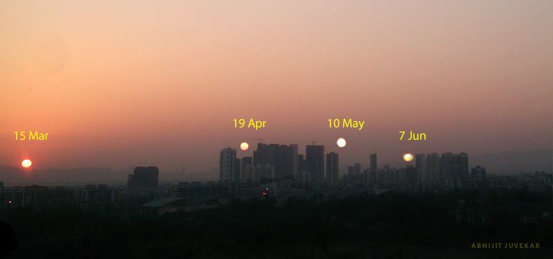
The sunset has been making its way north, as illustrated in this 2016 photo composite by Abhijit Juvekar.

The June solstice – your signal to celebrate summer in the Northern Hemisphere and winter in the Southern Hemisphere – will happen on June 21, 2019, at 15:54 UTC. That’s 10:54 a.m. CDT in North America on June 21. Translate UTC to your time. For us in the Northern Hemisphere, this solstice marks the longest day of the year. Early dawns. Long days. Late sunsets. Short nights. The sun at its height each day, as it crosses the sky. Meanwhile, south of the equator, winter begins.

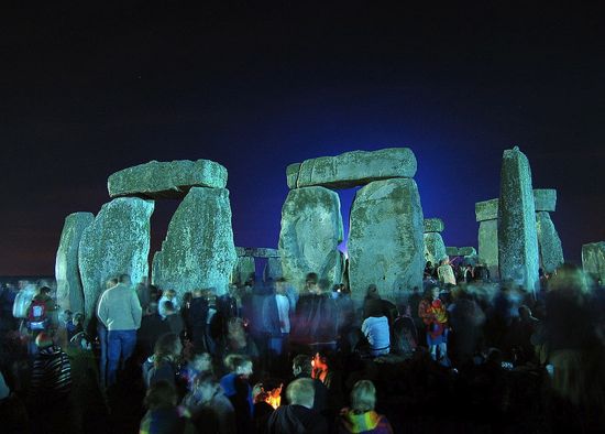
Waiting for dawn to arrive at Stonehenge, summer solstice 2005. Image via Andrew Dunn/Wikimedia Commons. Read more about summer solstice at Stonehenge.

What is a solstice? Ancient cultures knew that the sun’s path across the sky, the length of daylight, and the location of the sunrise and sunset all shifted in a regular way throughout the year.

They built monuments, such as Stonehenge, to follow the sun’s yearly progress.

Today, we know that the solstice is an astronomical event, caused by Earth’s tilt on its axis and its motion in orbit around the sun.

It’s because Earth doesn’t orbit upright. Instead, our world is tilted on its axis by 23 1/2 degrees. Earth’s Northern and Southern Hemispheres trade places in receiving the sun’s light and warmth most directly.

At the June solstice, Earth is positioned in its orbit so that our world’s North Pole is leaning most toward the sun. As seen from Earth, the sun is directly overhead at noon 23 1/2 degrees north of the equator, at an imaginary line encircling the globe known as the Tropic of Cancer – named after the constellation Cancer the Crab. This is as far north as the sun ever gets.

All locations north of the equator have days longer than 12 hours at the June solstice. Meanwhile, all locations south of the equator have days shorter than 12 hours.

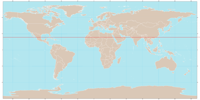
The red line shows the Tropic of Cancer. As seen from this line of latitude, the sun appears overhead at noon on the June solstice. Image via Wikimedia Commons.

When is the solstice where I live? The solstice takes place place on June 21, 2019, at 15:54 UTC. That’s 10:54 a.m. CDT in North America on June 21.

A solstice happens at the same instant for all of us, everywhere on Earth. To find the time of the solstice in your location, you have to translate to your time zone.

Here’s an example of how to do that. In the central United States, for those of us using Central Daylight Time, we subtract five hours from Universal Time. That’s how we get 10:54 a.m. CDT as the time of the 2019 June solstice (15:54 UTC on June 21 minus 5 equals 10:54 a.m. CDT on June 21).

Want to know the time in your location? Check out EarthSky’s article How to translate UTC to your time. And just remember: you’re translating from 15:54 UTC, June 21.

Sunset via EarthSky Facebook friend Lucy Bee in Dallas, Texas.

Where should I look to see signs of the solstice in nature? Everywhere. For all of Earth’s creatures, nothing is so fundamental as the length of the day. After all, the sun is the ultimate source of almost all light and warmth on Earth’s surface.

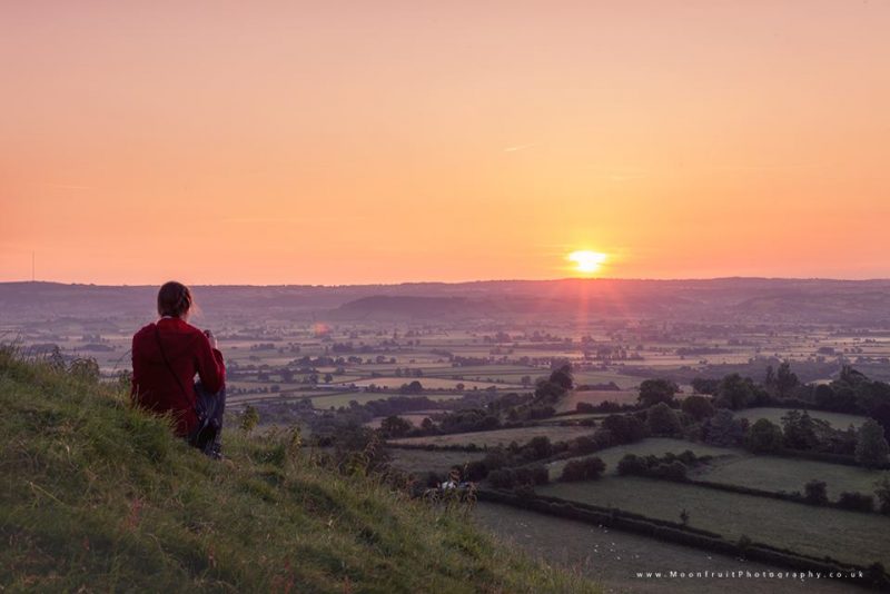
If you live in the Northern Hemisphere, you might notice the early dawns and late sunsets, and the high arc of the sun across the sky each day. You might see how high the sun appears in the sky at local noon. And be sure to look at your noontime shadow. Around the time of the solstice, it’s your shortest noontime shadow of the year.

If you’re a person who’s tuned in to the out-of-doors, you know the peaceful, comforting feeling that accompanies these signs and signals of the year’s longest day.

Watching the solstice sunrise. Photo via Sarah Little-Knitwitz, Glastonbury Tor, Somerset, U.K.

Is the solstice the first day of summer? No world body has designated an official day to start each new season, and different schools of thought or traditions define the seasons in different ways.

In meteorology, for example, summer begins on June 1. And every school child knows that summer starts when the last school bell of the year rings.

Yet June 21 is perhaps the most widely recognized day upon which summer begins in the Northern Hemisphere and upon which winter begins on the southern half of Earth’s globe. There’s nothing official about it, but it’s such a long-held tradition that we all recognize it to be so.

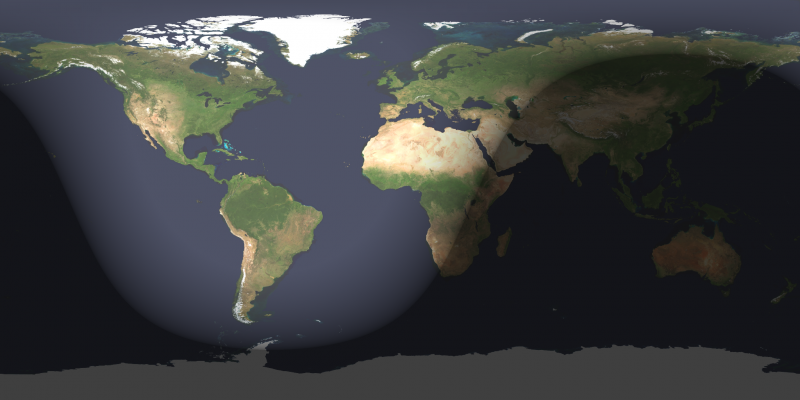
Worldwide map via the U.S. Naval Observatory shows the day and night sides of Earth at the instant of the June solstice (June 21, 2019, at 15:54 UTC).

It has been universal among humans to treasure this time of warmth and light.

For us in the modern world, the solstice is a time to recall the reverence and understanding that early people had for the sky. Some 5,000 years ago, people placed huge stones in a circle on a broad plain in what’s now England and aligned them with the June solstice sunrise.

We may never comprehend the full significance of Stonehenge. But we do know that knowledge of this sort wasn’t limited to just one part of the world. Around the same time Stonehenge was being constructed in England, two great pyramids and then the Sphinx were built on Egyptian sands. If you stood at the Sphinx on the summer solstice and gazed toward the two pyramids, you’d see the sun set exactly between them.

How does it end up hotter later in the summer, if June has the longest day? People often ask:

If the June solstice brings the longest day, why do we experience the hottest weather in late July and August?

This effect is called the lag of the seasons. It’s the same reason it’s hotter in mid-afternoon than at noontime. Earth just takes a while to warm up after a long winter. Even in June, ice and snow still blanket the ground in some places. The sun has to melt the ice – and warm the oceans – and then we feel the most sweltering summer heat.

Ice and snow have been melting since spring began. Meltwater and rainwater have been percolating down through snow on tops of glaciers.

But the runoff from glaciers isn’t as great now as it’ll be in another month, even though sunlight is striking the northern hemisphere most directly around now.

So wait another month for the hottest weather. It’ll come when the days are already beginning to shorten again, as Earth continues to move in orbit around the sun, bringing us closer to another winter.

And so the cycle continues.

Hello summer solstice!

Bottom line: The 2019 June solstice happens on June 21 at 15:54 UTC. That’s 10:54 a.m. CDT in North America. This solstice – which marks the beginning of summer in the Northern Hemisphere – marks the sun’s most northerly point in Earth’s sky. It’s an event celebrated by people throughout the ages.

Visit EarthSky Tonight for easy-to-use night sky charts and info. Updated daily.

Celebrate the summer solstice as the Chinese philosophers did

Why the hottest weather isn’t on the longest day

from EarthSky http://bit.ly/2XM8cXw

The sunset has been making its way north, as illustrated in this 2016 photo composite by Abhijit Juvekar.

The June solstice – your signal to celebrate summer in the Northern Hemisphere and winter in the Southern Hemisphere – will happen on June 21, 2019, at 15:54 UTC. That’s 10:54 a.m. CDT in North America on June 21. Translate UTC to your time. For us in the Northern Hemisphere, this solstice marks the longest day of the year. Early dawns. Long days. Late sunsets. Short nights. The sun at its height each day, as it crosses the sky. Meanwhile, south of the equator, winter begins.

Waiting for dawn to arrive at Stonehenge, summer solstice 2005. Image via Andrew Dunn/Wikimedia Commons. Read more about summer solstice at Stonehenge.

What is a solstice? Ancient cultures knew that the sun’s path across the sky, the length of daylight, and the location of the sunrise and sunset all shifted in a regular way throughout the year.

They built monuments, such as Stonehenge, to follow the sun’s yearly progress.

Today, we know that the solstice is an astronomical event, caused by Earth’s tilt on its axis and its motion in orbit around the sun.

It’s because Earth doesn’t orbit upright. Instead, our world is tilted on its axis by 23 1/2 degrees. Earth’s Northern and Southern Hemispheres trade places in receiving the sun’s light and warmth most directly.

At the June solstice, Earth is positioned in its orbit so that our world’s North Pole is leaning most toward the sun. As seen from Earth, the sun is directly overhead at noon 23 1/2 degrees north of the equator, at an imaginary line encircling the globe known as the Tropic of Cancer – named after the constellation Cancer the Crab. This is as far north as the sun ever gets.

All locations north of the equator have days longer than 12 hours at the June solstice. Meanwhile, all locations south of the equator have days shorter than 12 hours.

The red line shows the Tropic of Cancer. As seen from this line of latitude, the sun appears overhead at noon on the June solstice. Image via Wikimedia Commons.

When is the solstice where I live? The solstice takes place place on June 21, 2019, at 15:54 UTC. That’s 10:54 a.m. CDT in North America on June 21.

A solstice happens at the same instant for all of us, everywhere on Earth. To find the time of the solstice in your location, you have to translate to your time zone.

Here’s an example of how to do that. In the central United States, for those of us using Central Daylight Time, we subtract five hours from Universal Time. That’s how we get 10:54 a.m. CDT as the time of the 2019 June solstice (15:54 UTC on June 21 minus 5 equals 10:54 a.m. CDT on June 21).

Want to know the time in your location? Check out EarthSky’s article How to translate UTC to your time. And just remember: you’re translating from 15:54 UTC, June 21.

Sunset via EarthSky Facebook friend Lucy Bee in Dallas, Texas.

Where should I look to see signs of the solstice in nature? Everywhere. For all of Earth’s creatures, nothing is so fundamental as the length of the day. After all, the sun is the ultimate source of almost all light and warmth on Earth’s surface.

If you live in the Northern Hemisphere, you might notice the early dawns and late sunsets, and the high arc of the sun across the sky each day. You might see how high the sun appears in the sky at local noon. And be sure to look at your noontime shadow. Around the time of the solstice, it’s your shortest noontime shadow of the year.

If you’re a person who’s tuned in to the out-of-doors, you know the peaceful, comforting feeling that accompanies these signs and signals of the year’s longest day.

Watching the solstice sunrise. Photo via Sarah Little-Knitwitz, Glastonbury Tor, Somerset, U.K.

Is the solstice the first day of summer? No world body has designated an official day to start each new season, and different schools of thought or traditions define the seasons in different ways.

In meteorology, for example, summer begins on June 1. And every school child knows that summer starts when the last school bell of the year rings.

Yet June 21 is perhaps the most widely recognized day upon which summer begins in the Northern Hemisphere and upon which winter begins on the southern half of Earth’s globe. There’s nothing official about it, but it’s such a long-held tradition that we all recognize it to be so.

Worldwide map via the U.S. Naval Observatory shows the day and night sides of Earth at the instant of the June solstice (June 21, 2019, at 15:54 UTC).

It has been universal among humans to treasure this time of warmth and light.

For us in the modern world, the solstice is a time to recall the reverence and understanding that early people had for the sky. Some 5,000 years ago, people placed huge stones in a circle on a broad plain in what’s now England and aligned them with the June solstice sunrise.

We may never comprehend the full significance of Stonehenge. But we do know that knowledge of this sort wasn’t limited to just one part of the world. Around the same time Stonehenge was being constructed in England, two great pyramids and then the Sphinx were built on Egyptian sands. If you stood at the Sphinx on the summer solstice and gazed toward the two pyramids, you’d see the sun set exactly between them.

How does it end up hotter later in the summer, if June has the longest day? People often ask:

If the June solstice brings the longest day, why do we experience the hottest weather in late July and August?

This effect is called the lag of the seasons. It’s the same reason it’s hotter in mid-afternoon than at noontime. Earth just takes a while to warm up after a long winter. Even in June, ice and snow still blanket the ground in some places. The sun has to melt the ice – and warm the oceans – and then we feel the most sweltering summer heat.

Ice and snow have been melting since spring began. Meltwater and rainwater have been percolating down through snow on tops of glaciers.

But the runoff from glaciers isn’t as great now as it’ll be in another month, even though sunlight is striking the northern hemisphere most directly around now.

So wait another month for the hottest weather. It’ll come when the days are already beginning to shorten again, as Earth continues to move in orbit around the sun, bringing us closer to another winter.

And so the cycle continues.

Hello summer solstice!

Bottom line: The 2019 June solstice happens on June 21 at 15:54 UTC. That’s 10:54 a.m. CDT in North America. This solstice – which marks the beginning of summer in the Northern Hemisphere – marks the sun’s most northerly point in Earth’s sky. It’s an event celebrated by people throughout the ages.

Visit EarthSky Tonight for easy-to-use night sky charts and info. Updated daily.

Celebrate the summer solstice as the Chinese philosophers did

Why the hottest weather isn’t on the longest day

from EarthSky http://bit.ly/2XM8cXw

Venus at sunrise from ISS

View larger. | Venus – brightest planet visible in Earth’s sky – is the little dot in the lower center-left of this image by astronaut Christina Koch. The blue line is Earth’s atmosphere, appearing to shimmer from the vantage point of the orbiting space station.

From the International Space Station (ISS), NASA astronaut Christina Koch snapped and posted this image of the planet Venus at sunrise on May 31, 2019.

From Earth at this same time, Venus could be seen in the morning sky, in the east before sunup. It’s still in Earth’s morning sky, getting close to the sunrise, not easy to see anymore, especially from Earth’s Northern Hemisphere (it’s a bit easier to see from the southern part of Earth). Venus will be lost in the sun’s glare for all of us sometime around early July. It’ll pass behind the sun at superior conjunction on August 14. We’ll see Venus next in the evening sky sometime in September.

Read more: EarthSky’s guide to the visible planets

Bottom line: Photo of Venus at sunrise on May 31, 2019, taken by an astronaut aboard the ISS.

Via NASA

from EarthSky http://bit.ly/2KUv3wv

View larger. | Venus – brightest planet visible in Earth’s sky – is the little dot in the lower center-left of this image by astronaut Christina Koch. The blue line is Earth’s atmosphere, appearing to shimmer from the vantage point of the orbiting space station.

From the International Space Station (ISS), NASA astronaut Christina Koch snapped and posted this image of the planet Venus at sunrise on May 31, 2019.

From Earth at this same time, Venus could be seen in the morning sky, in the east before sunup. It’s still in Earth’s morning sky, getting close to the sunrise, not easy to see anymore, especially from Earth’s Northern Hemisphere (it’s a bit easier to see from the southern part of Earth). Venus will be lost in the sun’s glare for all of us sometime around early July. It’ll pass behind the sun at superior conjunction on August 14. We’ll see Venus next in the evening sky sometime in September.

Read more: EarthSky’s guide to the visible planets

Bottom line: Photo of Venus at sunrise on May 31, 2019, taken by an astronaut aboard the ISS.

Via NASA

from EarthSky http://bit.ly/2KUv3wv

Montauk lighthouse at dawn

Fred Lingen captured this early sunrise silhouette of the Montauk lighthouse in Montauk, New York, on June 5, 2019.

from EarthSky http://bit.ly/31wfv7K

Fred Lingen captured this early sunrise silhouette of the Montauk lighthouse in Montauk, New York, on June 5, 2019.

from EarthSky http://bit.ly/31wfv7K

Earliest sunrises before summer solstice

Top of post: June sunrise in Sea Bright, New Jersey, via Steve Scanlon Photography.

At mid-northern latitudes in the Northern Hemisphere, your earliest sunrises of the year happen around mid-June. That’s despite the fact that the summer solstice – and the year’s longest day – are still about a week away. And if you live at middle latitudes in the Southern Hemisphere, your earliest sunsets take place around now, even though the winter solstice – your shortest day – isn’t for another week.

For the Northern Hemisphere: Even if you’re not an early riser, this is a super month for an early morning walk. The dawn light is beautiful at this time of year.

For the Southern Hemisphere: If you’re someone who relishes the day’s light, as many do, you’ll be glad to know the sunsets will soon be shifting later!

Early sunrise in Sweden via Per Ola Wiberg.

The exact date of earliest sunrise (and earliest sunset) varies with latitude. At 40 degrees north latitude – the latitude of, say, Philadelphia in Pennsylvania – the earliest sunrise of the year will happen on June 14. For that same latitude, the latest sunset of the year will fall on or near June 27. Meanwhile, the longest day of the year – the day containing the greatest amount of daylight, overall – comes on the solstice on June 21.

So it is for other Northern Hemisphere latitudes. The dates of earliest sunrise and latest sunset don’t coincide exactly with the solstice. Appreciably south of Philadelphia’s latitude, the earliest sunrise has already come and gone (in late May or early June) and the latest sunset occurs at a later date (sometimes as late as July). In Hawaii, for instance, the earliest sunrise precedes the June solstice by about two weeks, and the latest sunset comes about two weeks after. Farther north, the earliest sunrise and latest sunset happen closer to the June solstice. Check it out at your latitude, using links on our almanac page.

The earliest sunrises come before the summer solstice because the day is more than 24 hours long at this time of the year. In the Southern Hemisphere, the earliest sunsets of the year come before the winter solstice for the same reason.

Enjoying EarthSky so far? Sign up for our free daily newsletter today!

View larger. | June sunrise over Currituck, North Carolina. Image via Greg Diesel Walck – Lunar/Landscape Photographer.

In June, the day (as measured by successive returns of the midday sun) is nearly 1/4 minute longer than 24 hours. Hence, the midday sun (solar noon) comes later by the clock on the June solstice than it does one week before. Therefore, the sunrise and sunset times also come later by the clock, as the tables below help to explain.

For Philadelphia (40 degrees north latitude)

Date	Sunrise	Midday (Solar Noon)	Sunset	Daylight Hours
June 14	5:31 a.m.	1:00 p.m.	8:30 p.m.	14h 59m 09s
June 21	5:32 a.m.	1:02 p.m.	8:32 p.m.	15h 00m 33s

For Valdivia, Chile (40 degrees south latitude)

Date	Sunrise	Midday (Solar Noon)	Sunset	Daylight Hours
June 14	8:12 a.m.	12:53 p.m.	5:34 p.m.	9h 22m 01s
June 21	8:14 a.m.	12:54 p.m.	5:35 p.m.	9h 20m 33s

Source: timeanddate.com.

The primary reason for the earliest sunrise preceding the summer solstice (and the earliest sunset preceding the winter solstice) is the inclination of the Earth’s rotational axis. The earliest sunrise or sunset would take place before the solstice even if the Earth went around the sun in a circular orbit.

However, the Earth’s elliptical orbit does affect the severity of the phenomenon. At the June solstice, Earth in its orbit is rather close to aphelion – its farthest point from the sun – which lessens the effect. At the December solstice, Earth is rather close to perihelion – its closest point to the sun – which accentuates it.

At middle latitudes, the earliest sunrise/sunset comes about one week before the June summer/winter solstice, and the latest sunset/sunrise about one week after the June solstice.

Yet, at the other end of the year, at middle latitudes, the earliest sunset/sunrise comes about two weeks before the December winter/summer solstice, and the latest sunrise/sunset about two weeks after the December solstice.

Early sunrise by Flickr user Rafal Zieba.

Bottom line: Are you an early riser? If so – if you live in the Northern Hemisphere – you might know your earliest sunrises of the year are happening now. Southern Hemisphere? Your earliest sunsets are around now.

EarthSky astronomy kits are perfect for beginners. Order today from the EarthSky store

Donate: Your support means the world to us

from EarthSky http://bit.ly/31tPSV3

Top of post: June sunrise in Sea Bright, New Jersey, via Steve Scanlon Photography.

At mid-northern latitudes in the Northern Hemisphere, your earliest sunrises of the year happen around mid-June. That’s despite the fact that the summer solstice – and the year’s longest day – are still about a week away. And if you live at middle latitudes in the Southern Hemisphere, your earliest sunsets take place around now, even though the winter solstice – your shortest day – isn’t for another week.

For the Northern Hemisphere: Even if you’re not an early riser, this is a super month for an early morning walk. The dawn light is beautiful at this time of year.

For the Southern Hemisphere: If you’re someone who relishes the day’s light, as many do, you’ll be glad to know the sunsets will soon be shifting later!

Early sunrise in Sweden via Per Ola Wiberg.

The exact date of earliest sunrise (and earliest sunset) varies with latitude. At 40 degrees north latitude – the latitude of, say, Philadelphia in Pennsylvania – the earliest sunrise of the year will happen on June 14. For that same latitude, the latest sunset of the year will fall on or near June 27. Meanwhile, the longest day of the year – the day containing the greatest amount of daylight, overall – comes on the solstice on June 21.

So it is for other Northern Hemisphere latitudes. The dates of earliest sunrise and latest sunset don’t coincide exactly with the solstice. Appreciably south of Philadelphia’s latitude, the earliest sunrise has already come and gone (in late May or early June) and the latest sunset occurs at a later date (sometimes as late as July). In Hawaii, for instance, the earliest sunrise precedes the June solstice by about two weeks, and the latest sunset comes about two weeks after. Farther north, the earliest sunrise and latest sunset happen closer to the June solstice. Check it out at your latitude, using links on our almanac page.

The earliest sunrises come before the summer solstice because the day is more than 24 hours long at this time of the year. In the Southern Hemisphere, the earliest sunsets of the year come before the winter solstice for the same reason.

Enjoying EarthSky so far? Sign up for our free daily newsletter today!

View larger. | June sunrise over Currituck, North Carolina. Image via Greg Diesel Walck – Lunar/Landscape Photographer.

In June, the day (as measured by successive returns of the midday sun) is nearly 1/4 minute longer than 24 hours. Hence, the midday sun (solar noon) comes later by the clock on the June solstice than it does one week before. Therefore, the sunrise and sunset times also come later by the clock, as the tables below help to explain.

For Philadelphia (40 degrees north latitude)

Date	Sunrise	Midday (Solar Noon)	Sunset	Daylight Hours
June 14	5:31 a.m.	1:00 p.m.	8:30 p.m.	14h 59m 09s
June 21	5:32 a.m.	1:02 p.m.	8:32 p.m.	15h 00m 33s

For Valdivia, Chile (40 degrees south latitude)

Date	Sunrise	Midday (Solar Noon)	Sunset	Daylight Hours
June 14	8:12 a.m.	12:53 p.m.	5:34 p.m.	9h 22m 01s
June 21	8:14 a.m.	12:54 p.m.	5:35 p.m.	9h 20m 33s

Source: timeanddate.com.

The primary reason for the earliest sunrise preceding the summer solstice (and the earliest sunset preceding the winter solstice) is the inclination of the Earth’s rotational axis. The earliest sunrise or sunset would take place before the solstice even if the Earth went around the sun in a circular orbit.

However, the Earth’s elliptical orbit does affect the severity of the phenomenon. At the June solstice, Earth in its orbit is rather close to aphelion – its farthest point from the sun – which lessens the effect. At the December solstice, Earth is rather close to perihelion – its closest point to the sun – which accentuates it.

At middle latitudes, the earliest sunrise/sunset comes about one week before the June summer/winter solstice, and the latest sunset/sunrise about one week after the June solstice.

Yet, at the other end of the year, at middle latitudes, the earliest sunset/sunrise comes about two weeks before the December winter/summer solstice, and the latest sunrise/sunset about two weeks after the December solstice.

Early sunrise by Flickr user Rafal Zieba.

Bottom line: Are you an early riser? If so – if you live in the Northern Hemisphere – you might know your earliest sunrises of the year are happening now. Southern Hemisphere? Your earliest sunsets are around now.

EarthSky astronomy kits are perfect for beginners. Order today from the EarthSky store

Donate: Your support means the world to us

from EarthSky http://bit.ly/31tPSV3

A focus on fathers: The science of dads

Anthropologist James Rilling with his son Toby, 8, and daughter Mia, 2. (Photo by Becky Stein)

Want to do something special for a father on June 16? Try asking him what he finds most rewarding — and most challenging — about being a dad.

James Rilling, an anthropologist at Emory University, recently completed in-depth interviews on that topic with 120 new fathers. Rilling and his colleague Craig Hadley, also an anthropologist at Emory, are still analyzing data from the interviews for a comprehensive study.

One result, however, is already clear. A positive-and-negative-affect scale administered to the subjects before and after the interviews shows how talking about fatherhood influenced their moods. “Most of them experienced an increase in how enthusiastic, proud and inspired they felt after talking about their experience as a father,” Rilling says. “They seemed to find it therapeutic to talk about their feelings surrounding being a father, particularly if they were struggling with some things. The challenges of being a mother are often much greater. So fathers may think that nobody really wants to hear about the things they are dealing with as a new parent.”

Read more about Rilling's work here, and learn five surprising facts about fathers.

Related:
How dads bond with toddlers
Dads show gender biases

from eScienceCommons http://bit.ly/2X9MzDf

Anthropologist James Rilling with his son Toby, 8, and daughter Mia, 2. (Photo by Becky Stein)

Want to do something special for a father on June 16? Try asking him what he finds most rewarding — and most challenging — about being a dad.

James Rilling, an anthropologist at Emory University, recently completed in-depth interviews on that topic with 120 new fathers. Rilling and his colleague Craig Hadley, also an anthropologist at Emory, are still analyzing data from the interviews for a comprehensive study.

One result, however, is already clear. A positive-and-negative-affect scale administered to the subjects before and after the interviews shows how talking about fatherhood influenced their moods. “Most of them experienced an increase in how enthusiastic, proud and inspired they felt after talking about their experience as a father,” Rilling says. “They seemed to find it therapeutic to talk about their feelings surrounding being a father, particularly if they were struggling with some things. The challenges of being a mother are often much greater. So fathers may think that nobody really wants to hear about the things they are dealing with as a new parent.”

Read more about Rilling's work here, and learn five surprising facts about fathers.

Related:
How dads bond with toddlers
Dads show gender biases

from eScienceCommons http://bit.ly/2X9MzDf

US astronomers speak on SpaceX Starlink satellites

An image of the NGC 5353/4 galaxy group made with a telescope at Lowell Observatory in Arizona, USA, on the night of May 25, 2019. The diagonal lines running across the image are trails of reflected light left by more than 25 of the 60 recently launched Starlink satellites as they passed through the telescope’s field of view. Although this image serves as an illustration of the impact of reflections from satellite constellations, please note that the density of these satellites is significantly higher in the days after launch (as seen here) than they will be when they reach their final orbits. Following their initial orbits, the satellites will diminish in brightness as they are boosted to a final orbital altitude. How bright will they ultimately be? That’s as yet unclear. Image via Victoria Girgis/Lowell Observatory.

On May 23, 2019, entrepreneur Elon Musk’s company SpaceX launched 60 Starlink communication satellites aboard a single rocket. Within days, skywatchers worldwide spotted them flying in formation as they orbited Earth and reflected sunlight from their shiny metal surfaces. Some people, unaware that artificial satellites can be seen moving against the starry background every clear night, reported UFO sightings. Astronomers, on the other hand, knew exactly what they were seeing … and immediately began to worry.

SpaceX had suggested that the satellites would be visible just barely, if at all. But – in the days after launch – the Starlink constellation shone as brightly as many astronomical constellations, and SpaceX intends to launch approximately 12,000 of these spacecraft as part of an effort to provide internet service to everyone in the world. Megan Donahue, of Michigan State University, is president of the American Astronomical Society (AAS). She said in a statement:

I think it’s commendable and very impressive engineering to spread the information and opportunities made possible by internet access, but I, like many astronomers, am very worried about the future of these new bright satellites.

The Starlink satellites and similar swarms being developed by other companies could eventually outnumber the visible stars in our night sky.

A view of SpaceX’s first 60 Starlink satellites in orbit, still in stacked configuration, with the Earth as a brilliant blue backdrop on May 23, 2019. Image via SpaceX/ Space.com.

The primary professional organization for U.S. astronomers is the American Astronomical Society (AAS). Among other activities, this group hosts twice-yearly meetings of astronomers across the nation. On June 8, 2019, at the 234th AAS meeting in St. Louis, Missouri, the AAS Board of Trustees adopted the following position statement on satellite constellations:

The American Astronomical Society notes with concern the impending deployment of very large constellations of satellites into Earth orbit. The number of such satellites is projected to grow into the tens of thousands over the next several years, creating the potential for substantial adverse impacts to ground- and space-based astronomy. These impacts could include significant disruption of optical and near-infrared observations by direct detection of satellites in reflected and emitted light; contamination of radio astronomical observations by electromagnetic radiation in satellite communication bands; and collision with space-based observatories.

The AAS recognizes that outer space is an increasingly available resource with many possible uses. However, the potential for multiple large satellite constellations to adversely affect both each other and the study of the cosmos is becoming increasingly apparent, both in low Earth orbit and beyond.

The AAS is actively working to assess the impacts on astronomy of large satellite constellations before their numbers rise further. Only with thorough and quantitative understanding can we properly assess the risks and identify appropriate mitigating actions. The AAS desires that this be a collaborative effort among its members, other scientific societies, and other space stakeholders including private companies. The AAS will support and facilitate the work by relevant parties to understand fully and minimize the impact of large satellite constellations on ground- and space-based astronomy.

Jeffrey C. Hall, of Lowell Observatory, is Chair of the AAS Committee on Light Pollution, Radio Interference, and Space Debris. Hall said:

The natural night sky is a resource not just for astronomers but for all who look upward to understand and enjoy the splendor of the universe, and its degradation has many negative impacts beyond the astronomical.

I appreciate the initial conversation we have already had with SpaceX, and I look forward to working with my AAS colleagues and with all stakeholders to understand and mitigate the effects of the rapidly increasing numbers of satellites in near-Earth orbit.

Donahue added:

I’m looking forward to productive conversations between astronomers and SpaceX. I fully expect that we will come up with creative solutions that can serve as models for other companies to follow.

Bottom line: At its June 2019 meeting, the American Astronomical Society – chief professional organization for astronomers in the U.S. – issued a position statement about the SpaceX starlink satellites. It said, in part: “The AAS is actively working to assess the impacts on astronomy of large satellite constellations before their numbers rise further.”

Read more: Wow! The SpaceX Starlink satellite train

Via American Astronomical Society

from EarthSky http://bit.ly/31kMkEC

An image of the NGC 5353/4 galaxy group made with a telescope at Lowell Observatory in Arizona, USA, on the night of May 25, 2019. The diagonal lines running across the image are trails of reflected light left by more than 25 of the 60 recently launched Starlink satellites as they passed through the telescope’s field of view. Although this image serves as an illustration of the impact of reflections from satellite constellations, please note that the density of these satellites is significantly higher in the days after launch (as seen here) than they will be when they reach their final orbits. Following their initial orbits, the satellites will diminish in brightness as they are boosted to a final orbital altitude. How bright will they ultimately be? That’s as yet unclear. Image via Victoria Girgis/Lowell Observatory.

On May 23, 2019, entrepreneur Elon Musk’s company SpaceX launched 60 Starlink communication satellites aboard a single rocket. Within days, skywatchers worldwide spotted them flying in formation as they orbited Earth and reflected sunlight from their shiny metal surfaces. Some people, unaware that artificial satellites can be seen moving against the starry background every clear night, reported UFO sightings. Astronomers, on the other hand, knew exactly what they were seeing … and immediately began to worry.

SpaceX had suggested that the satellites would be visible just barely, if at all. But – in the days after launch – the Starlink constellation shone as brightly as many astronomical constellations, and SpaceX intends to launch approximately 12,000 of these spacecraft as part of an effort to provide internet service to everyone in the world. Megan Donahue, of Michigan State University, is president of the American Astronomical Society (AAS). She said in a statement:

I think it’s commendable and very impressive engineering to spread the information and opportunities made possible by internet access, but I, like many astronomers, am very worried about the future of these new bright satellites.

The Starlink satellites and similar swarms being developed by other companies could eventually outnumber the visible stars in our night sky.

A view of SpaceX’s first 60 Starlink satellites in orbit, still in stacked configuration, with the Earth as a brilliant blue backdrop on May 23, 2019. Image via SpaceX/ Space.com.

The primary professional organization for U.S. astronomers is the American Astronomical Society (AAS). Among other activities, this group hosts twice-yearly meetings of astronomers across the nation. On June 8, 2019, at the 234th AAS meeting in St. Louis, Missouri, the AAS Board of Trustees adopted the following position statement on satellite constellations:

The American Astronomical Society notes with concern the impending deployment of very large constellations of satellites into Earth orbit. The number of such satellites is projected to grow into the tens of thousands over the next several years, creating the potential for substantial adverse impacts to ground- and space-based astronomy. These impacts could include significant disruption of optical and near-infrared observations by direct detection of satellites in reflected and emitted light; contamination of radio astronomical observations by electromagnetic radiation in satellite communication bands; and collision with space-based observatories.

The AAS recognizes that outer space is an increasingly available resource with many possible uses. However, the potential for multiple large satellite constellations to adversely affect both each other and the study of the cosmos is becoming increasingly apparent, both in low Earth orbit and beyond.

The AAS is actively working to assess the impacts on astronomy of large satellite constellations before their numbers rise further. Only with thorough and quantitative understanding can we properly assess the risks and identify appropriate mitigating actions. The AAS desires that this be a collaborative effort among its members, other scientific societies, and other space stakeholders including private companies. The AAS will support and facilitate the work by relevant parties to understand fully and minimize the impact of large satellite constellations on ground- and space-based astronomy.

Jeffrey C. Hall, of Lowell Observatory, is Chair of the AAS Committee on Light Pollution, Radio Interference, and Space Debris. Hall said:

The natural night sky is a resource not just for astronomers but for all who look upward to understand and enjoy the splendor of the universe, and its degradation has many negative impacts beyond the astronomical.

I appreciate the initial conversation we have already had with SpaceX, and I look forward to working with my AAS colleagues and with all stakeholders to understand and mitigate the effects of the rapidly increasing numbers of satellites in near-Earth orbit.

Donahue added:

I’m looking forward to productive conversations between astronomers and SpaceX. I fully expect that we will come up with creative solutions that can serve as models for other companies to follow.

Bottom line: At its June 2019 meeting, the American Astronomical Society – chief professional organization for astronomers in the U.S. – issued a position statement about the SpaceX starlink satellites. It said, in part: “The AAS is actively working to assess the impacts on astronomy of large satellite constellations before their numbers rise further.”

Read more: Wow! The SpaceX Starlink satellite train

Via American Astronomical Society

from EarthSky http://bit.ly/31kMkEC

Climate change: sea level rise could displace millions of people within two generations

Jonathan Bamber, Professor of Physical Geography, University of Bristol and Michael Oppenheimer, Professor of Geosciences and International Affairs, Princeton University

This article is republished from The Conversation under a Creative Commons license. Read the original article.

Antarctica is further from civilization than any other place on Earth. The Greenland ice sheet is closer to home but around one tenth the size of its southern sibling. Together, these two ice masses hold enough frozen water to raise global mean sea level by 65 metres if they were to suddenly melt. But how likely is this to happen?

The Antarctic ice sheet is around one and half times larger than Australia. What’s happening in one part of Antarctica may not be the same as what’s happening in another – just like the east and west coasts of the US can experience very different responses to, for example, a change in the El Niño weather pattern. These are periodic climate events that result in wetter conditions across the southern US, warmer conditions in the north and drier weather on the north-eastern seaboard.

The ice in Antarctica is nearly 5km thick in places and we have very little idea what the conditions are like at the base, even though those conditions play a key role in determining the speed with which the ice can respond to climate change, including how fast it can flow toward and into the ocean. A warm, wet base lubricates the bedrock of land beneath the ice and allows it to slide over it.

Though invisible from the surface, melting within the ice can speed up the process by which ice sheets slide towards the sea. Gans33/Shutterstock

These issues have made it particularly difficult to produce model simulations of how ice sheets will respond to climate change in future. Models have to capture all the processes and uncertainties that we know about and those that we don’t – the “known unknowns” and the “unknown unknowns” as Donald Rumsfeld once put it. As a result, several recent studies suggest that previous Intergovernmental Panel on Climate Change reports may have underestimated how much melting ice sheets will contribute to sea level in future.

What the experts say

Fortunately, models are not the only tools for predicting the future. Structured Expert Judgement is a method from a study one of us published in 2013. Experts give their judgement on a hard-to-model problem and their judgements are combined in a way that takes into account how good they are at assessing their own uncertainty. This provides a rational consensus.

The approach has been used when the consequences of an event are potentially catastrophic, but our ability to model the system is poor. These include volcanic eruptions, earthquakes, the spread of vector-borne diseases such as malaria and even aeroplane crashes.

Since the study in 2013, scientists modelling ice sheets have improved their models by trying to incorporate processes that cause positive and negative feedback. Impurities on the surface of the Greenland ice sheet cause positive feedback as they enhance melting by absorbing more of the sun’s heat. The stabilising effect of bedrock rising as the overlying ice thins, lessening the weight on the bed, is an example of negative feedback, as it slows the rate that the ice melts.

The record of observations of ice sheet change, primarily from satellite data, has also grown in length and quality, helping to improve knowledge of the recent behaviour of the ice sheets.

With colleagues from the UK and US, we undertook a new Structured Expert Judgement exercise. With all the new research, data and knowledge, you might expect the uncertainties around how much ice sheet melting will contribute to sea level rise to have got smaller. Unfortunately, that’s not what we found. What we did find was a range of future outcomes that go from bad to worse.

Reconstructed sea level for the last 2500 years. Note the marked increase in rate since about 1900 that is unprecedented over the whole time period. Robert Kopp/Kopp et al. (2016), Author provided

Rising uncertainty

We gathered together 22 experts in the US and UK in 2018 and combined their judgements. The results are sobering. Rather than a shrinking in the uncertainty of future ice sheet behaviour over the last six years, it has grown.

If the global temperature increase stays below 2°C, the experts’ best estimate of the average contribution of the ice sheets to sea level was 26cm. They concluded, however, that there is a 5% chance that the contribution could be as much as 80cm.

If this is combined with the two other main factors that influence sea level – glaciers melting around the world and the expansion of ocean water as it warms – then global mean sea level rise could exceed one metre by 2100. If this were to occur, many small island states would experience their current once-in-a-hundred–year flood every other day and become effectively uninhabitable.

A climate refugee crisis could dwarf all previous forced migrations. Punghi/Shutterstock

For a climate change scenario closer to business as usual – where our current trajectory for economic growth continues and global temperatures increase by 5℃ – the outlook is even more bleak. The experts’ best estimate average in this case is 51cm of sea level rise caused by melting ice sheets by 2100, but with a 5% chance that global sea level rise could exceed two metres by 2100. That has the potential to displace some 200m people.

Let’s try and put this into context. The Syrian refugee crisis is estimated to have caused about a million people to migrate to Europe. This occurred over years rather than a century, giving much less time for countries to adjust. Still, sea level rise driven by migration of this size might threaten the existence of nation states and result in unimaginable stress on resources and space. There is time to change course, but not much, and the longer we delay the harder it gets, the bigger the mountain we have to climb.

 

from Skeptical Science http://bit.ly/2KcHow9

Jonathan Bamber, Professor of Physical Geography, University of Bristol and Michael Oppenheimer, Professor of Geosciences and International Affairs, Princeton University

This article is republished from The Conversation under a Creative Commons license. Read the original article.

Antarctica is further from civilization than any other place on Earth. The Greenland ice sheet is closer to home but around one tenth the size of its southern sibling. Together, these two ice masses hold enough frozen water to raise global mean sea level by 65 metres if they were to suddenly melt. But how likely is this to happen?

The Antarctic ice sheet is around one and half times larger than Australia. What’s happening in one part of Antarctica may not be the same as what’s happening in another – just like the east and west coasts of the US can experience very different responses to, for example, a change in the El Niño weather pattern. These are periodic climate events that result in wetter conditions across the southern US, warmer conditions in the north and drier weather on the north-eastern seaboard.

The ice in Antarctica is nearly 5km thick in places and we have very little idea what the conditions are like at the base, even though those conditions play a key role in determining the speed with which the ice can respond to climate change, including how fast it can flow toward and into the ocean. A warm, wet base lubricates the bedrock of land beneath the ice and allows it to slide over it.

Though invisible from the surface, melting within the ice can speed up the process by which ice sheets slide towards the sea. Gans33/Shutterstock

These issues have made it particularly difficult to produce model simulations of how ice sheets will respond to climate change in future. Models have to capture all the processes and uncertainties that we know about and those that we don’t – the “known unknowns” and the “unknown unknowns” as Donald Rumsfeld once put it. As a result, several recent studies suggest that previous Intergovernmental Panel on Climate Change reports may have underestimated how much melting ice sheets will contribute to sea level in future.

What the experts say

Fortunately, models are not the only tools for predicting the future. Structured Expert Judgement is a method from a study one of us published in 2013. Experts give their judgement on a hard-to-model problem and their judgements are combined in a way that takes into account how good they are at assessing their own uncertainty. This provides a rational consensus.

The approach has been used when the consequences of an event are potentially catastrophic, but our ability to model the system is poor. These include volcanic eruptions, earthquakes, the spread of vector-borne diseases such as malaria and even aeroplane crashes.

Since the study in 2013, scientists modelling ice sheets have improved their models by trying to incorporate processes that cause positive and negative feedback. Impurities on the surface of the Greenland ice sheet cause positive feedback as they enhance melting by absorbing more of the sun’s heat. The stabilising effect of bedrock rising as the overlying ice thins, lessening the weight on the bed, is an example of negative feedback, as it slows the rate that the ice melts.

The record of observations of ice sheet change, primarily from satellite data, has also grown in length and quality, helping to improve knowledge of the recent behaviour of the ice sheets.

With colleagues from the UK and US, we undertook a new Structured Expert Judgement exercise. With all the new research, data and knowledge, you might expect the uncertainties around how much ice sheet melting will contribute to sea level rise to have got smaller. Unfortunately, that’s not what we found. What we did find was a range of future outcomes that go from bad to worse.

Reconstructed sea level for the last 2500 years. Note the marked increase in rate since about 1900 that is unprecedented over the whole time period. Robert Kopp/Kopp et al. (2016), Author provided

Rising uncertainty

We gathered together 22 experts in the US and UK in 2018 and combined their judgements. The results are sobering. Rather than a shrinking in the uncertainty of future ice sheet behaviour over the last six years, it has grown.

If the global temperature increase stays below 2°C, the experts’ best estimate of the average contribution of the ice sheets to sea level was 26cm. They concluded, however, that there is a 5% chance that the contribution could be as much as 80cm.

If this is combined with the two other main factors that influence sea level – glaciers melting around the world and the expansion of ocean water as it warms – then global mean sea level rise could exceed one metre by 2100. If this were to occur, many small island states would experience their current once-in-a-hundred–year flood every other day and become effectively uninhabitable.

A climate refugee crisis could dwarf all previous forced migrations. Punghi/Shutterstock

For a climate change scenario closer to business as usual – where our current trajectory for economic growth continues and global temperatures increase by 5℃ – the outlook is even more bleak. The experts’ best estimate average in this case is 51cm of sea level rise caused by melting ice sheets by 2100, but with a 5% chance that global sea level rise could exceed two metres by 2100. That has the potential to displace some 200m people.

Let’s try and put this into context. The Syrian refugee crisis is estimated to have caused about a million people to migrate to Europe. This occurred over years rather than a century, giving much less time for countries to adjust. Still, sea level rise driven by migration of this size might threaten the existence of nation states and result in unimaginable stress on resources and space. There is time to change course, but not much, and the longer we delay the harder it gets, the bigger the mountain we have to climb.

 

from Skeptical Science http://bit.ly/2KcHow9

Lobbying against key US climate regulation ‘cost society $60bn’, study finds

This is a re-post from Carbon Brief by Josh Gabbatiss

Political lobbying in the US that helped block the progress of proposed climate regulation a decade ago led to a social cost of $60bn, according to a new study.

Environmental economists Dr Kyle Meng and Dr Ashwin Rode have produced what they believe is the first attempt to quantify the toll such anti-climate lobbying efforts take on society.

The pair say their work reveals the power firms can have in curtailing government action on climate change, in the face of “overwhelming evidence” that its social benefits outweigh the costs, which range from reduced farming yields to lower GDP.

Crucially, they found that the various fossil-fuel and transport companies expecting to emerge as “losers” after the bill were more effective lobbyists than those expecting gains.

The authors say their results, published in Nature Climate Change, support the conclusion that lobbying is partly responsible for the scarcity of climate regulations being enacted around the world.

However, they tell Carbon Brief that there is still hope for those seeking to develop effective new climate policies:

“Our bottom line is: climate policy emerges from a political process. We’ve shown that this political process can undermine the chances of passing climate policy. But we’ve also shown that careful design of climate policy can help make it more politically robust to opposition.”

Waxman-Markey

The Waxman-Markey bill, described by the study’s authors as “the most prominent and promising US climate regulation so far”, did not make it past the Senate in 2010, meaning it never passed into law.

However, having passed the House of Representatives in summer 2009, it remains the closest the nation has ever come to implementing wide-ranging climate legislation.

Formally known as the American Clean Energy and Security Act 2009, the bill proposed a 17% cut in US emissions by 2020 – and then 80% by 2050 – based on 2005 levels. It was named after the two Democrat representatives who wrote it, Henry Waxman and Edward Markey.

A key element of Waxman-Markey was its cap-and-trade scheme, which would have limited the amount of greenhouse gases produced nationally while creating a fixed number of tradable emission permits for industry nationwide. Other measures included a renewable energy standard and legislation for energy efficiency and grid modernisation.

The bill was the culmination of several attempts stretching back to 2003 to pass cap-and-trade legislation limiting the US economy’s emissions. As none of these efforts were successful, president Barack Obama instead relied on the executive powers of the US Environmental Protection Agency to tackle greenhouse gas emissions, specifically its power to regulate “any pollutant” that “endangers public health or welfare”.

Today, with climate change low on the list of federal priorities, there are some state-level ventures in place, such as California’s cap-and-trade system, but still no country-wide scheme.

Climate lobbying

Media reports around the time Waxman-Markey was making its way through the US government made it clear that lobbyists were thought to be hindering its progress.

However, the authors of the new paper note that despite such reporting it is difficult to appreciate the extent of political lobbying and its impact on the final outcome. According to them, lobbying often goes unrecorded and, even when it is, it can prove difficult to quantify which groups stand to gain and lose – and to what extent.

For Waxman–Markey, they made use of the “comprehensive US congressional lobbying record” to piece together a full picture of the situation at the time.

According to their paper, the bill accounted for around 14% of all recorded lobbying expenditures at the time – more spending on lobbying than for any other policy between 2000 and 2016.

A separate study conducted by Dr Robert Brulle of Drexel University in 2018 found that over this period, climate issues took up roughly 4% of all lobbying spend, amounting to over £2bn. He concluded that fossil-fuel, transport and utility companies dominated this activity, with expenditures that “dwarfed” those of environmental groups and renewable energy corporations.

However, some of the highest spenders listed by Meng and Rode in their new paper were those who stood to gain from the bill, such as General Electric and the Pacific Gas and Electric Company.

Winners and losers

To understand different lobbyists’ motivations, the researchers first had to work out how Waxman-Markey would have affected companies had it passed into law.

They took data on prices from a prediction market tied to the bill while it was being considered by government and combined it with stock prices for firms involved in lobbying. In a joint email, Meng and Rode explain how this works to Carbon Brief:

“A prediction market is essentially a betting market where participants bet on the likelihood of some event happening. Think of it like a sports betting market (in other words, will Liverpool win the Champions League final?), but you can do that for any event…The power of a prediction market is that, under some standard economic assumptions, the price of a bet of that market at any point in time reflects the market-held belief that the event will happen.”

Their “innovation”, the pair explain, was to combine this information with the stock market prices of publicly listed firms that lobbied on the bill. They were then able to estimate how the values of publicly listed firms were expected to change if the policy had passed.

One benefit of this approach was that it allowed them to establish, in what they describe as a “hands-off”, objective manner, who the “winners” and “losers” were in the face of climate regulations. This allowed the researchers to bypass both their own preconceptions, as well as any statements made by the firms themselves which, as the pair point out, may not be reliable.

The team found a statistically significant relationship [see graph below] between how much a firm spent on Waxman-Markey lobbying and how much the bill was expected to change its stock value.

The researchers found a significant relationship between the amount a firm spent lobbying on Waxman-Markey (x-axis) and how much the policy was expected to alter its stock value (y-axis). Source: Meng and Rode (2019).

To then understand how these activities affected the final outcome, they built a model that incorporated a game-theory approach to lobbying – where firms try to influence policy for their own benefit – and a standard model of how firms behave under a cap-and-trade policy.

This model revealed that oppositional lobbying – that is to say activities by companies that stood to lose out – was the most effective. This implies the input of “loser” firms, which include Boeing, Marathon Oil, Walmart and Ford, had more influence that “winners”, despite spending comparable sums on lobbying. From this conclusion, the researchers estimated that the sum of all lobbying decreased the probability of the bill being enacted by 13%.

While their work does not resolve the issue of why this disparity between winners and losers exists, the pair tell Carbon Brief they have some ideas:

“The asymmetric effectiveness could be due to differential abilities of firms to collectively organise, gather information on policy consequences and to lobby on other, related issues. While all these explanations are consistent with our findings, data limitations prevent us from examining which one is most relevant for the Waxman-Markey bill.”

Social cost

To pin down the financial impact of lobbying, the researchers built on previous research that placed a $467bn (in 2018 US dollars) price tag on the global social cost of the failed Waxman-Markey bill. This was based on forecasts of greenhouse gas emissions that would have been avoided had it come into force.

The cost of these emissions for the world as a whole are well established, as they explain to Carbon Brief:

“A large body of research has demonstrated the costs of unmitigated climate change in myriad contexts, including decreased agricultural yields, increased conflict, increased mortality and morbidity, decreased labor supply, and lower gross domestic product. Failure to enact Waxman-Markey is expected to have had adverse consequence in all these areas by allowing for higher greenhouse gas emissions and thus higher climate damages.”

Since they found that lobbying increased the likelihood of the bill not passing by 13%, they assigned this share of the total cost to lobbying efforts. This gave them their final figure of $60bn.

Given the current state of climate policy in the US, Meng and Rode conclude by suggesting how this knowledge could be used to build a new strategy that is more likely to be successful.

They took their model and used it to gauge the impact of providing more free credits under the cap-and-trade system to companies – and particularly those that lobbied against the new bill. As this would lead to greater gains or reduced losses, they found it could effectively reduce the amount of anti-bill lobbying and make it more likely to succeed.

While they note such actions could prove unpopular and have unintended political consequences, they suggest this information could nevertheless be incorporated into future policy-making. They tell Carbon Brief:

“Our new point is that if the very likelihood of having climate policy enacted in the first place may be jeopardised by political influences (via lobbying), why not try to use this revenue to neutralise some of the political opposition in a targeted way.”

 

Meng, K.C. and Rode, A. (2019) The social cost of lobbying over climate policy, Nature Climate Change, www.nature.com/articles/s41558-019-0489-6

from Skeptical Science http://bit.ly/2KbXUMX

This is a re-post from Carbon Brief by Josh Gabbatiss

Political lobbying in the US that helped block the progress of proposed climate regulation a decade ago led to a social cost of $60bn, according to a new study.

Environmental economists Dr Kyle Meng and Dr Ashwin Rode have produced what they believe is the first attempt to quantify the toll such anti-climate lobbying efforts take on society.

The pair say their work reveals the power firms can have in curtailing government action on climate change, in the face of “overwhelming evidence” that its social benefits outweigh the costs, which range from reduced farming yields to lower GDP.

Crucially, they found that the various fossil-fuel and transport companies expecting to emerge as “losers” after the bill were more effective lobbyists than those expecting gains.

The authors say their results, published in Nature Climate Change, support the conclusion that lobbying is partly responsible for the scarcity of climate regulations being enacted around the world.

However, they tell Carbon Brief that there is still hope for those seeking to develop effective new climate policies:

“Our bottom line is: climate policy emerges from a political process. We’ve shown that this political process can undermine the chances of passing climate policy. But we’ve also shown that careful design of climate policy can help make it more politically robust to opposition.”

Waxman-Markey

The Waxman-Markey bill, described by the study’s authors as “the most prominent and promising US climate regulation so far”, did not make it past the Senate in 2010, meaning it never passed into law.

However, having passed the House of Representatives in summer 2009, it remains the closest the nation has ever come to implementing wide-ranging climate legislation.

Formally known as the American Clean Energy and Security Act 2009, the bill proposed a 17% cut in US emissions by 2020 – and then 80% by 2050 – based on 2005 levels. It was named after the two Democrat representatives who wrote it, Henry Waxman and Edward Markey.

A key element of Waxman-Markey was its cap-and-trade scheme, which would have limited the amount of greenhouse gases produced nationally while creating a fixed number of tradable emission permits for industry nationwide. Other measures included a renewable energy standard and legislation for energy efficiency and grid modernisation.

The bill was the culmination of several attempts stretching back to 2003 to pass cap-and-trade legislation limiting the US economy’s emissions. As none of these efforts were successful, president Barack Obama instead relied on the executive powers of the US Environmental Protection Agency to tackle greenhouse gas emissions, specifically its power to regulate “any pollutant” that “endangers public health or welfare”.

Today, with climate change low on the list of federal priorities, there are some state-level ventures in place, such as California’s cap-and-trade system, but still no country-wide scheme.

Climate lobbying

Media reports around the time Waxman-Markey was making its way through the US government made it clear that lobbyists were thought to be hindering its progress.

However, the authors of the new paper note that despite such reporting it is difficult to appreciate the extent of political lobbying and its impact on the final outcome. According to them, lobbying often goes unrecorded and, even when it is, it can prove difficult to quantify which groups stand to gain and lose – and to what extent.

For Waxman–Markey, they made use of the “comprehensive US congressional lobbying record” to piece together a full picture of the situation at the time.

According to their paper, the bill accounted for around 14% of all recorded lobbying expenditures at the time – more spending on lobbying than for any other policy between 2000 and 2016.

A separate study conducted by Dr Robert Brulle of Drexel University in 2018 found that over this period, climate issues took up roughly 4% of all lobbying spend, amounting to over £2bn. He concluded that fossil-fuel, transport and utility companies dominated this activity, with expenditures that “dwarfed” those of environmental groups and renewable energy corporations.

However, some of the highest spenders listed by Meng and Rode in their new paper were those who stood to gain from the bill, such as General Electric and the Pacific Gas and Electric Company.

Winners and losers

To understand different lobbyists’ motivations, the researchers first had to work out how Waxman-Markey would have affected companies had it passed into law.

They took data on prices from a prediction market tied to the bill while it was being considered by government and combined it with stock prices for firms involved in lobbying. In a joint email, Meng and Rode explain how this works to Carbon Brief:

“A prediction market is essentially a betting market where participants bet on the likelihood of some event happening. Think of it like a sports betting market (in other words, will Liverpool win the Champions League final?), but you can do that for any event…The power of a prediction market is that, under some standard economic assumptions, the price of a bet of that market at any point in time reflects the market-held belief that the event will happen.”

Their “innovation”, the pair explain, was to combine this information with the stock market prices of publicly listed firms that lobbied on the bill. They were then able to estimate how the values of publicly listed firms were expected to change if the policy had passed.

One benefit of this approach was that it allowed them to establish, in what they describe as a “hands-off”, objective manner, who the “winners” and “losers” were in the face of climate regulations. This allowed the researchers to bypass both their own preconceptions, as well as any statements made by the firms themselves which, as the pair point out, may not be reliable.

The team found a statistically significant relationship [see graph below] between how much a firm spent on Waxman-Markey lobbying and how much the bill was expected to change its stock value.

The researchers found a significant relationship between the amount a firm spent lobbying on Waxman-Markey (x-axis) and how much the policy was expected to alter its stock value (y-axis). Source: Meng and Rode (2019).

To then understand how these activities affected the final outcome, they built a model that incorporated a game-theory approach to lobbying – where firms try to influence policy for their own benefit – and a standard model of how firms behave under a cap-and-trade policy.

This model revealed that oppositional lobbying – that is to say activities by companies that stood to lose out – was the most effective. This implies the input of “loser” firms, which include Boeing, Marathon Oil, Walmart and Ford, had more influence that “winners”, despite spending comparable sums on lobbying. From this conclusion, the researchers estimated that the sum of all lobbying decreased the probability of the bill being enacted by 13%.

While their work does not resolve the issue of why this disparity between winners and losers exists, the pair tell Carbon Brief they have some ideas:

“The asymmetric effectiveness could be due to differential abilities of firms to collectively organise, gather information on policy consequences and to lobby on other, related issues. While all these explanations are consistent with our findings, data limitations prevent us from examining which one is most relevant for the Waxman-Markey bill.”

Social cost

To pin down the financial impact of lobbying, the researchers built on previous research that placed a $467bn (in 2018 US dollars) price tag on the global social cost of the failed Waxman-Markey bill. This was based on forecasts of greenhouse gas emissions that would have been avoided had it come into force.

The cost of these emissions for the world as a whole are well established, as they explain to Carbon Brief:

“A large body of research has demonstrated the costs of unmitigated climate change in myriad contexts, including decreased agricultural yields, increased conflict, increased mortality and morbidity, decreased labor supply, and lower gross domestic product. Failure to enact Waxman-Markey is expected to have had adverse consequence in all these areas by allowing for higher greenhouse gas emissions and thus higher climate damages.”

Since they found that lobbying increased the likelihood of the bill not passing by 13%, they assigned this share of the total cost to lobbying efforts. This gave them their final figure of $60bn.

Given the current state of climate policy in the US, Meng and Rode conclude by suggesting how this knowledge could be used to build a new strategy that is more likely to be successful.

They took their model and used it to gauge the impact of providing more free credits under the cap-and-trade system to companies – and particularly those that lobbied against the new bill. As this would lead to greater gains or reduced losses, they found it could effectively reduce the amount of anti-bill lobbying and make it more likely to succeed.

While they note such actions could prove unpopular and have unintended political consequences, they suggest this information could nevertheless be incorporated into future policy-making. They tell Carbon Brief:

“Our new point is that if the very likelihood of having climate policy enacted in the first place may be jeopardised by political influences (via lobbying), why not try to use this revenue to neutralise some of the political opposition in a targeted way.”

 

Meng, K.C. and Rode, A. (2019) The social cost of lobbying over climate policy, Nature Climate Change, www.nature.com/articles/s41558-019-0489-6

from Skeptical Science http://bit.ly/2KbXUMX

Moon and Spica on June 11 and 12

On June 11 and 12, 2019, use the waxing gibbous moon to find Spica, the brightest star in the constellation Virgo the Maiden. In fact, Spica is Virgo’s one and only 1st-magnitude star. Although the bright moon will wipe out a number of fainter stars from the canopy of night tonight, bright Spica should withstand the moonlit glare. If you have trouble seeing Spica, place your finger over the moon and look for a bright star nearby.

We in the Northern Hemisphere associate the star Spica with the spring and summer seasons. That’s because Spica first lights up the early evening sky in late March or early April, and then disappears from the evening sky around the September equinox.

The constellation Virgo stands as a memorial to that old legend of Hades, god of the underworld, who was said to have abducted Persephone, daughter of Demeter, goddess of the harvest. According to the legend, Hades took Persephone to his underground hideaway. Demeter’s grief was so great that she abandoned her role in insuring fruitfulness and fertility. In some parts of the globe, it’s said, winter cold came out of season and turned the once-verdant Earth in to a frigid wasteland. Elsewhere, summer heat was said to scorch the Earth and give rise to pestilence and disease. According to the myth, Earth would not bear fruit again until Demeter was reunited with her daughter.

Zeus, the king of the gods, intervened, insisting that Persephone be returned to her mother. However, Persephone was instructed to abstain from food until the reunion with her mother was a done deal. Alas, Hades purposely gave Persephone a pomegranate to take along, knowing she would eat a few seeds on her way home. Because of Persephone’s slip-up, Persephone has to return to the underworld for a number of months each year. When she does so, Demeter grieves, and winter reigns.

The constellation Virgo is linked to Demeter (and also Ishtar of Babylonian mythology, Isis of Egyptian mythology and Ceres of Roman mythology). Virgo is seen as a Maiden, associated with the harvest and fertility. The Latin word spicum refers to the ear of wheat Virgo holds in her left hand. The star Spica takes its name from this ear of wheat. Each evening, if you watch at the same time, you’ll see Spica slowly shift westward, toward the sunset direction. Eventually, Spica will get so close to the sunset that’ll fade in the glare of evening twilight. Once Spica disappears from the evening sky, we at northerly latitudes must harvest our crops and put away firewood, because the cold winter season is on its way.

We are surrounded by stars. Because Earth orbits in a flat plane around the sun, we see the sun against the same stars again and again throughout the year. Those constellations, which have been special to people throughout the ages, are the constellations of the Zodiac. Image via Professor Marcia Rieke.

The constellations of the zodiac – like Virgo – define the sun’s path across our sky. Putting it another way, each year, the sun passes in front of all the constellations of the zodiac. This year, 2019, the sun leaves the constellation Leo to enter the constellation Virgo on September 17, 2019. Then the sun leaves the constellation Virgo to enter the constellation Libra on October 31, 2019 (Halloween).

Three other 1st-magnitude zodiacal stars join up with Spica to help sky gazers to envision the ecliptic – the sun’s annual path in front of the backdrop stars: Aldebaran, Regulus, Spica, Antares and Aldebaran. Every year, the sun has its annual conjunction with Aldebaran on or near June 1, Regulus on or near August 23, Spica around mid-October, and Antares on or near December 1.

Of course, all these stars are invisible on their conjunction dates with the sun because they are totally lost in the sun’s glare at that time. However, six months before or after these stars’ conjunction dates, these stars are out all night long. Six months one way or the other of their conjunction, these stars reside opposite the sun in the sky and therefore stay out all night (Regulus around February 23, Spica around mid-April, Antares around June 1 and Aldebaran around December 1).

The ecliptic – Earth’s orbital plane projected onto the constellations of the zodiac – crosses the celestial equator (declination of O degrees) in the constellation Virgo. Because Spica resides so close to the ecliptic, it is considered a major star of the zodiac. Virgo constellation chart via the International Astronomical Union (IAU).

Bottom line: Use the moon to see the star Spica at nightfall on June 11 and 12, 2019, and celebrate this star’s presence in the evening sky.

from EarthSky http://bit.ly/2KHI2S4

On June 11 and 12, 2019, use the waxing gibbous moon to find Spica, the brightest star in the constellation Virgo the Maiden. In fact, Spica is Virgo’s one and only 1st-magnitude star. Although the bright moon will wipe out a number of fainter stars from the canopy of night tonight, bright Spica should withstand the moonlit glare. If you have trouble seeing Spica, place your finger over the moon and look for a bright star nearby.

We in the Northern Hemisphere associate the star Spica with the spring and summer seasons. That’s because Spica first lights up the early evening sky in late March or early April, and then disappears from the evening sky around the September equinox.

The constellation Virgo stands as a memorial to that old legend of Hades, god of the underworld, who was said to have abducted Persephone, daughter of Demeter, goddess of the harvest. According to the legend, Hades took Persephone to his underground hideaway. Demeter’s grief was so great that she abandoned her role in insuring fruitfulness and fertility. In some parts of the globe, it’s said, winter cold came out of season and turned the once-verdant Earth in to a frigid wasteland. Elsewhere, summer heat was said to scorch the Earth and give rise to pestilence and disease. According to the myth, Earth would not bear fruit again until Demeter was reunited with her daughter.

Zeus, the king of the gods, intervened, insisting that Persephone be returned to her mother. However, Persephone was instructed to abstain from food until the reunion with her mother was a done deal. Alas, Hades purposely gave Persephone a pomegranate to take along, knowing she would eat a few seeds on her way home. Because of Persephone’s slip-up, Persephone has to return to the underworld for a number of months each year. When she does so, Demeter grieves, and winter reigns.

The constellation Virgo is linked to Demeter (and also Ishtar of Babylonian mythology, Isis of Egyptian mythology and Ceres of Roman mythology). Virgo is seen as a Maiden, associated with the harvest and fertility. The Latin word spicum refers to the ear of wheat Virgo holds in her left hand. The star Spica takes its name from this ear of wheat. Each evening, if you watch at the same time, you’ll see Spica slowly shift westward, toward the sunset direction. Eventually, Spica will get so close to the sunset that’ll fade in the glare of evening twilight. Once Spica disappears from the evening sky, we at northerly latitudes must harvest our crops and put away firewood, because the cold winter season is on its way.

We are surrounded by stars. Because Earth orbits in a flat plane around the sun, we see the sun against the same stars again and again throughout the year. Those constellations, which have been special to people throughout the ages, are the constellations of the Zodiac. Image via Professor Marcia Rieke.

The constellations of the zodiac – like Virgo – define the sun’s path across our sky. Putting it another way, each year, the sun passes in front of all the constellations of the zodiac. This year, 2019, the sun leaves the constellation Leo to enter the constellation Virgo on September 17, 2019. Then the sun leaves the constellation Virgo to enter the constellation Libra on October 31, 2019 (Halloween).

Three other 1st-magnitude zodiacal stars join up with Spica to help sky gazers to envision the ecliptic – the sun’s annual path in front of the backdrop stars: Aldebaran, Regulus, Spica, Antares and Aldebaran. Every year, the sun has its annual conjunction with Aldebaran on or near June 1, Regulus on or near August 23, Spica around mid-October, and Antares on or near December 1.

Of course, all these stars are invisible on their conjunction dates with the sun because they are totally lost in the sun’s glare at that time. However, six months before or after these stars’ conjunction dates, these stars are out all night long. Six months one way or the other of their conjunction, these stars reside opposite the sun in the sky and therefore stay out all night (Regulus around February 23, Spica around mid-April, Antares around June 1 and Aldebaran around December 1).

The ecliptic – Earth’s orbital plane projected onto the constellations of the zodiac – crosses the celestial equator (declination of O degrees) in the constellation Virgo. Because Spica resides so close to the ecliptic, it is considered a major star of the zodiac. Virgo constellation chart via the International Astronomical Union (IAU).

Bottom line: Use the moon to see the star Spica at nightfall on June 11 and 12, 2019, and celebrate this star’s presence in the evening sky.

from EarthSky http://bit.ly/2KHI2S4

IAU invites countries to name exoplanets

Artist’s concept of a landscape on an exoplanet, or planet orbiting a distant star. There are now more than 4,000 known exoplanets, according to some counts. Image via IAU.

Reprinted from an International Astronomical Union (IAU) statement published June 6, 2019

Within the framework of its 100th anniversary commemorations, the International Astronomical Union (IAU) is organizing the IAU100 NameExoWorlds global campaign that allows any country in the world to give a popular name to a selected exoplanet and its host star. Nearly 100 countries have already signed up to organize national campaigns that will provide the public with an opportunity to vote. The aim of this initiative is to create awareness of our place in the universe and to reflect on how the Earth would potentially be perceived by a civilisation on another planet.

In recent years, astronomers have discovered thousands of planets and planetary systems orbiting around nearby stars. Some are small and rocky like the Earth, while others are gas giants like Jupiter. It is now believed that most stars in the universe could have planets orbiting them and that some of them may have physical characteristics that resemble those of the Earth. The sheer number of stars in the universe, each potentially with orbiting planets, along with the ubiquity of prebiotic compounds, suggests that extraterrestrial life may be likely.

The IAU is the authority responsible for assigning official designations and names to celestial bodies [Editor’s Note: The IAU has claimed the right to be the arbiter of planetary and satellite nomenclature since its inception in 1919]. Now, while celebrating its first 100 years of fostering international collaboration (IAU100), it wishes to contribute to the fraternity of all people with a significant token of global identity. Following the first NameExoWorlds campaign, which named 31 exoplanets in 19 planetary systems in 2015, the IAU will now, within the framework of the IAU100 NameExoWorlds project, offer every country the chance to name one planetary system, comprising an exoplanet and its host star. Each nation’s designated star is visible from that country, and sufficiently bright to be observed through small telescopes …

Debra Elmegreen, IAU President Elect, said:

This exciting event invites everyone worldwide to think about their collective place in the universe, while stimulating creativity and global citizenship. The NameExoWorlds initiative reminds us that we are all together under one sky.

After carefully selecting a large sample of well-studied, confirmed exoplanets [*see note below] and their host stars, the IAU100 NameExoWorlds Steering Committee assigned a star-planet system to each country, taking account of the association with the country and the visibility of the host star from most of the country.

In each participating country, a national committee has been specially created by the National Outreach Coordinators (IAU NOCs) to carry out the campaign at the national level. The national committee, following the methodology and guidelines set up by the IAU100 NameExoWorlds Steering Committee, is the body responsible for providing the conditions for public participation, disseminating the project in the country and establishing a voting system.

The national campaigns will be carried out from June to November 2019 and, after final validation by the IAU100 NameExoWorlds Steering Committee, the global results will be announced in December 2019. The winning names will be used freely in parallel with the existing scientific nomenclature, with due credit to the persons that proposed them.

If your country is not yet organizing a national campaign, and you are part of a science organization or Non-Governmental Organization interested in carrying out a nationwide contest, there is still time until July 30, 2019, to express interest in organizing a national campaign. Send us your brief proposal through this form and the NameExoWorlds Steering Committee will review your proposal and will get back to you with its decision. Questions about national campaigns should be specifically addressed to the National Committees.

*Note: The NameExoWorlds campaign has selected planetary systems for naming composed of planets orbiting stars that could be observed with a small telescope from the latitude of the capital of each country. The system often has a link with the assigned country, such as the facilities used to discover the planet, or the scientists involved in the discovery of the planet. The existence of the planet is generally more secure for systems which were discovered earlier, as they have had more years of research to survive further scrutiny. For this reason, the sample is focused on exoplanets revealed during the first two decades of exoplanet exploration, with most discovery dates before 2012. The visual brightnesses range between 6th and 12th magnitude. The planets were all discovered via either the Doppler spectroscopy (radial velocity) method or transit method, and all were discovered using ground-based telescopes. The planets are all likely to be gas giants similar to Jupiter and Saturn, with estimated masses between 10 percent and 500 percent that of Jupiter. All these systems are composed of single stars with only one known planet orbiting around them. It is possible that the stars have additional planetary and stellar companions which may be discovered in the future. This is so that each country has an equal opportunity of naming similar celestial bodies.

View larger. | Artist’s concept depicting how common planets are around stars in our Milky Way galaxy. The planets, their orbits and their host stars are all vastly magnified compared to their real separations. Planets around stars are likely the rule rather than the exception. The average number of planets per star is greater than one. Image via ESO/M. Kornmesser.

Bottom line: The International Astronomical Union (IAU) is organizing the IAU100 NameExoWorlds global campaign that allows any country in the world to give a popular name to a selected exoplanet and its host star.

from EarthSky http://bit.ly/2WuoOBE

Artist’s concept of a landscape on an exoplanet, or planet orbiting a distant star. There are now more than 4,000 known exoplanets, according to some counts. Image via IAU.

Reprinted from an International Astronomical Union (IAU) statement published June 6, 2019

Within the framework of its 100th anniversary commemorations, the International Astronomical Union (IAU) is organizing the IAU100 NameExoWorlds global campaign that allows any country in the world to give a popular name to a selected exoplanet and its host star. Nearly 100 countries have already signed up to organize national campaigns that will provide the public with an opportunity to vote. The aim of this initiative is to create awareness of our place in the universe and to reflect on how the Earth would potentially be perceived by a civilisation on another planet.

In recent years, astronomers have discovered thousands of planets and planetary systems orbiting around nearby stars. Some are small and rocky like the Earth, while others are gas giants like Jupiter. It is now believed that most stars in the universe could have planets orbiting them and that some of them may have physical characteristics that resemble those of the Earth. The sheer number of stars in the universe, each potentially with orbiting planets, along with the ubiquity of prebiotic compounds, suggests that extraterrestrial life may be likely.

The IAU is the authority responsible for assigning official designations and names to celestial bodies [Editor’s Note: The IAU has claimed the right to be the arbiter of planetary and satellite nomenclature since its inception in 1919]. Now, while celebrating its first 100 years of fostering international collaboration (IAU100), it wishes to contribute to the fraternity of all people with a significant token of global identity. Following the first NameExoWorlds campaign, which named 31 exoplanets in 19 planetary systems in 2015, the IAU will now, within the framework of the IAU100 NameExoWorlds project, offer every country the chance to name one planetary system, comprising an exoplanet and its host star. Each nation’s designated star is visible from that country, and sufficiently bright to be observed through small telescopes …

Debra Elmegreen, IAU President Elect, said:

This exciting event invites everyone worldwide to think about their collective place in the universe, while stimulating creativity and global citizenship. The NameExoWorlds initiative reminds us that we are all together under one sky.

After carefully selecting a large sample of well-studied, confirmed exoplanets [*see note below] and their host stars, the IAU100 NameExoWorlds Steering Committee assigned a star-planet system to each country, taking account of the association with the country and the visibility of the host star from most of the country.

In each participating country, a national committee has been specially created by the National Outreach Coordinators (IAU NOCs) to carry out the campaign at the national level. The national committee, following the methodology and guidelines set up by the IAU100 NameExoWorlds Steering Committee, is the body responsible for providing the conditions for public participation, disseminating the project in the country and establishing a voting system.

The national campaigns will be carried out from June to November 2019 and, after final validation by the IAU100 NameExoWorlds Steering Committee, the global results will be announced in December 2019. The winning names will be used freely in parallel with the existing scientific nomenclature, with due credit to the persons that proposed them.

If your country is not yet organizing a national campaign, and you are part of a science organization or Non-Governmental Organization interested in carrying out a nationwide contest, there is still time until July 30, 2019, to express interest in organizing a national campaign. Send us your brief proposal through this form and the NameExoWorlds Steering Committee will review your proposal and will get back to you with its decision. Questions about national campaigns should be specifically addressed to the National Committees.

*Note: The NameExoWorlds campaign has selected planetary systems for naming composed of planets orbiting stars that could be observed with a small telescope from the latitude of the capital of each country. The system often has a link with the assigned country, such as the facilities used to discover the planet, or the scientists involved in the discovery of the planet. The existence of the planet is generally more secure for systems which were discovered earlier, as they have had more years of research to survive further scrutiny. For this reason, the sample is focused on exoplanets revealed during the first two decades of exoplanet exploration, with most discovery dates before 2012. The visual brightnesses range between 6th and 12th magnitude. The planets were all discovered via either the Doppler spectroscopy (radial velocity) method or transit method, and all were discovered using ground-based telescopes. The planets are all likely to be gas giants similar to Jupiter and Saturn, with estimated masses between 10 percent and 500 percent that of Jupiter. All these systems are composed of single stars with only one known planet orbiting around them. It is possible that the stars have additional planetary and stellar companions which may be discovered in the future. This is so that each country has an equal opportunity of naming similar celestial bodies.

View larger. | Artist’s concept depicting how common planets are around stars in our Milky Way galaxy. The planets, their orbits and their host stars are all vastly magnified compared to their real separations. Planets around stars are likely the rule rather than the exception. The average number of planets per star is greater than one. Image via ESO/M. Kornmesser.

Bottom line: The International Astronomical Union (IAU) is organizing the IAU100 NameExoWorlds global campaign that allows any country in the world to give a popular name to a selected exoplanet and its host star.

from EarthSky http://bit.ly/2WuoOBE

Will evidence for life on Mars look like fettuccine pasta?

An example of the “fettuccine” rocks at Mammoth Hot Springs in Wyoming, part of Yellowstone National Park. The pasta-like filaments are created by bacteria and appear completely unique from other rock formations. Image via Bruce Fouke.

What is the best way to search for life on Mars? Looking for fossils? Microbes, either past or present? It turns out that the best thing to look for might indeed be microbial, but not in a form most people would expect. The most obvious evidence for ancient Martian life might be … pasta? Fettucine specifically, but not the kind you eat, of course. Rather, scientists suggest looking for a certain type of rock formation that resembles fettuccine. On Earth at least, these sorts of rocks are known to be created only by microbes.

The new peer-reviewed paper outlining this intriguing possibility was published in the journal Astrobiology on April 30, 2019.

On Earth, these types of rock formations are created by bacteria that live in conditions a bit similar to those on Mars. According to University of Illinois geology professor Bruce Fouke, who led the new, NASA-funded study of such formations in Mammoth Hot Springs in Yellowstone National Park:

It has an unusual name, Sulfurihydrogenibium yellowstonense. We just call it ‘Sulfuri.’

Another view of the “fettuccine” rocks at Mammoth Hot Springs in Yellowstone National Park. Image via Bruce Fouke.

Closer view of the ends of the fettuccine-like strands. Image via Tom Murphy.

Crystalline rock formations are catalyzed by the bacteria in such a way that the rocks look like layers of fettuccine pasta. This unique morphology would make it quite easy to detect by rovers or landers on Mars. The strand-like appearance is a result of the Sulfuri bacteria latching onto one another in fast-moving water. As Fouke said:

They form tightly wound cables that wave like a flag that is fixed on one end. These Sulfuri cables look amazingly like fettuccine pasta, while further downstream they look more like capellini pasta.

The researchers even used sterilized pasta forks to take samples from the rock formations. Seems appropriate!

This bacterium is very ancient; it evolved prior to the oxygenation of Earth – the Great Oxidation Event, when a lot of oxygen was first added to the atmosphere – 2.35 billion years ago. It is also very tough, able to survive extremely hot, fast-flowing water bubbling up from underground hot springs. It can also withstand harsh ultraviolet light, which is the norm on Mars, and only lives in environments with little to no oxygen. It uses sulfur and carbon dioxide for energy. Mars also has extremely little oxygen in its atmosphere, and an abundance of carbon dioxide. Although it lives on Earth, this bacterium, or one similar to it, might be able to survive on Mars rather nicely. As Fouke said:

Taken together, these traits make it a prime candidate for colonizing Mars and other planets.

There is also another aspect of the fettuccine rock formations that helps to identify them as being created by life: proteins on the bacteria speed up the rate at which calcium carbonate – travertine – crystallizes in and around the cables about 1 billion times faster than in any other natural environment on Earth. The rock formations contain broad swaths of hardened rock with an undulating, filamentous organic-looking texture. As Fouke said:

This should be an easy form of fossilized life for a rover to detect on other planets.

Other kinds of microbial mats are also common on Earth, but these fettuccine-like ones are so unique that finding them on, say, Mars, would be pretty much solid evidence for life. According to Fouke:

If we see the deposition of this kind of extensive filamentous rock on other planets, we would know it’s a fingerprint of life. It’s big and it’s unique. No other rocks look like this. It would be definitive evidence of the presences of alien microbes.

Researchers involved in the new study. From left: Robert Sanford, professor of geology; Bruce Fouke, professor of geology; Kyle Fouke, undergraduate student at Bucknell University; Glenn Fried, director of core facilities, IGB; and Mayandi Sivaguru, associate director of core facilities IGB. Image via L. Brian Stauffer.

While this kind of fettuccine rocks has yet to be found on Mars, there have been other intriguing formations discovered by the Spirit and Curiosity rovers. There are cauliflower-like silica formations that resemble those made by microbes on Earth, in a region of ancient Martian hot springs in Gusev Crater, and possible microbial mats, identified by geobiologist Nora Noffke at Old Dominion University in Virginia, in sedimentary rocks that used to be at the bottom of a lake in Gale Crater. Similar formations to the cauliflower ones can also be found in Yellowstone National Park. The silica contains the fossilized remains of microorganisms. Sadly, Spirit died before it could investigate them further. The features seen by Curiosity look a lot like microbial mats, but unfortunately Curiosity isn’t equipped to make a definitive analysis. Neither of these curious formations have been proven to be evidence of life yet, but they are intriguing. As noted by Sherry Cady of the Pacific Northwest National Laboratory (PNNL):

Only when something that we have identified as a potential biosignature is proven to have been produced only by life, and not by any abiotic means, can we make the claim that definitive evidence for life has been found.

Bottom line: If you are searching for evidence of life on Mars, look for rock formations that resemble long, thin strands of fettuccine pasta. No, not from Martian chefs, but rather microbes that create these tell-tale signatures in rocks as they survive in very harsh conditions similar to those in hot springs on Earth.

Source: Physiology, Metabolism, and Fossilization of Hot-Spring Filamentous Microbial Mats

Via Illinois News Bureau

from EarthSky http://bit.ly/2XCL8dv

An example of the “fettuccine” rocks at Mammoth Hot Springs in Wyoming, part of Yellowstone National Park. The pasta-like filaments are created by bacteria and appear completely unique from other rock formations. Image via Bruce Fouke.

What is the best way to search for life on Mars? Looking for fossils? Microbes, either past or present? It turns out that the best thing to look for might indeed be microbial, but not in a form most people would expect. The most obvious evidence for ancient Martian life might be … pasta? Fettucine specifically, but not the kind you eat, of course. Rather, scientists suggest looking for a certain type of rock formation that resembles fettuccine. On Earth at least, these sorts of rocks are known to be created only by microbes.

The new peer-reviewed paper outlining this intriguing possibility was published in the journal Astrobiology on April 30, 2019.

On Earth, these types of rock formations are created by bacteria that live in conditions a bit similar to those on Mars. According to University of Illinois geology professor Bruce Fouke, who led the new, NASA-funded study of such formations in Mammoth Hot Springs in Yellowstone National Park:

It has an unusual name, Sulfurihydrogenibium yellowstonense. We just call it ‘Sulfuri.’

Another view of the “fettuccine” rocks at Mammoth Hot Springs in Yellowstone National Park. Image via Bruce Fouke.

Closer view of the ends of the fettuccine-like strands. Image via Tom Murphy.

Crystalline rock formations are catalyzed by the bacteria in such a way that the rocks look like layers of fettuccine pasta. This unique morphology would make it quite easy to detect by rovers or landers on Mars. The strand-like appearance is a result of the Sulfuri bacteria latching onto one another in fast-moving water. As Fouke said:

They form tightly wound cables that wave like a flag that is fixed on one end. These Sulfuri cables look amazingly like fettuccine pasta, while further downstream they look more like capellini pasta.

The researchers even used sterilized pasta forks to take samples from the rock formations. Seems appropriate!

This bacterium is very ancient; it evolved prior to the oxygenation of Earth – the Great Oxidation Event, when a lot of oxygen was first added to the atmosphere – 2.35 billion years ago. It is also very tough, able to survive extremely hot, fast-flowing water bubbling up from underground hot springs. It can also withstand harsh ultraviolet light, which is the norm on Mars, and only lives in environments with little to no oxygen. It uses sulfur and carbon dioxide for energy. Mars also has extremely little oxygen in its atmosphere, and an abundance of carbon dioxide. Although it lives on Earth, this bacterium, or one similar to it, might be able to survive on Mars rather nicely. As Fouke said:

Taken together, these traits make it a prime candidate for colonizing Mars and other planets.

There is also another aspect of the fettuccine rock formations that helps to identify them as being created by life: proteins on the bacteria speed up the rate at which calcium carbonate – travertine – crystallizes in and around the cables about 1 billion times faster than in any other natural environment on Earth. The rock formations contain broad swaths of hardened rock with an undulating, filamentous organic-looking texture. As Fouke said:

This should be an easy form of fossilized life for a rover to detect on other planets.

Other kinds of microbial mats are also common on Earth, but these fettuccine-like ones are so unique that finding them on, say, Mars, would be pretty much solid evidence for life. According to Fouke:

If we see the deposition of this kind of extensive filamentous rock on other planets, we would know it’s a fingerprint of life. It’s big and it’s unique. No other rocks look like this. It would be definitive evidence of the presences of alien microbes.

Researchers involved in the new study. From left: Robert Sanford, professor of geology; Bruce Fouke, professor of geology; Kyle Fouke, undergraduate student at Bucknell University; Glenn Fried, director of core facilities, IGB; and Mayandi Sivaguru, associate director of core facilities IGB. Image via L. Brian Stauffer.

While this kind of fettuccine rocks has yet to be found on Mars, there have been other intriguing formations discovered by the Spirit and Curiosity rovers. There are cauliflower-like silica formations that resemble those made by microbes on Earth, in a region of ancient Martian hot springs in Gusev Crater, and possible microbial mats, identified by geobiologist Nora Noffke at Old Dominion University in Virginia, in sedimentary rocks that used to be at the bottom of a lake in Gale Crater. Similar formations to the cauliflower ones can also be found in Yellowstone National Park. The silica contains the fossilized remains of microorganisms. Sadly, Spirit died before it could investigate them further. The features seen by Curiosity look a lot like microbial mats, but unfortunately Curiosity isn’t equipped to make a definitive analysis. Neither of these curious formations have been proven to be evidence of life yet, but they are intriguing. As noted by Sherry Cady of the Pacific Northwest National Laboratory (PNNL):

Only when something that we have identified as a potential biosignature is proven to have been produced only by life, and not by any abiotic means, can we make the claim that definitive evidence for life has been found.

Bottom line: If you are searching for evidence of life on Mars, look for rock formations that resemble long, thin strands of fettuccine pasta. No, not from Martian chefs, but rather microbes that create these tell-tale signatures in rocks as they survive in very harsh conditions similar to those in hot springs on Earth.

Source: Physiology, Metabolism, and Fossilization of Hot-Spring Filamentous Microbial Mats

Via Illinois News Bureau

from EarthSky http://bit.ly/2XCL8dv

Alphecca, the jewel in the Northern Crown

Corona Borealis, the Northern Crown, with its brightest star Alphecca, via Fred Espenak and AstroPixels. Used with permission.

Stars often have many names. You might hear people call the brightest star in the constellation Corona Borealis by any of these names: Alphecca, also called Gemma, also called Alpha Coronae Borealis or simply Alpha Cor Bor. The other proper name for Alphecca – Gemma – means gem or jewel. On a dark night under a dark sky, this star lives up to its name, sparkling at the forefront of the semicircle of stars that make up the constellation Corona Borealis, the Northern Crown. In the lore of the skies, this C-shaped constellation represents the crown or wreath worn by the ancient Minoan princess Ariadne.

Alphecca is brighter than the other stars in Corona Borealis, but only moderately bright in contrast to the brightest stars. It shines between summertime’s two most brilliant stars: Arcturus and Vega. An imaginary line drawn between these two brilliant beauties locates Alphecca every time, about one-third of the way from Arcturus to Vega.

As seen from mid-northern latitudes, Alphecca shines all night long – or nearly all night long – in April, May and June. Alphecca and this glittery bowl of stars crown the sky on July evenings, and continue to grace the heavens well into November. Starting around mid-November, Alphecca appears rather low in the west-northwest sky after dusk. It sets shortly after nightfall, then reappears in the east-northeast before dawn.

Alphecca is the brightest star in a C-shaped pattern of stars: the constellation Corona Borealis. It’s near the bright star Arcturus on the sky’s dome.

In the ancient Greek myth, the C-shaped pattern of our modern-day constellation Corona Borealis was sometimes considered to represent a crown that was given by Dionysus to Ariadne, a princess, daughter of Minos of Crete. When Ariadne married Dionysus – who was the Greek god of fertility and wine – she’s said to have worn the crown to her wedding. Later, Dionysus is said to have placed her crown in the heavens to commemorate the wedding.

The seven stars that make up Corona Borealis the Northern Crown are relatively faint and best seen in a dark sky. See Alphecca, brightest star in the C? Bright star below is Arcturus. Image via AlltheSky.com.

The star Alphecca is quite interesting in itself. Like the star Algol in the constellation Perseus, it is an eclipsing binary star, with an orbital period of about 17.4 days. In other words, on this timescale of only days, the fainter of Alphecca’s two component stars passes in front of the brighter one, resulting a slight dip in brightness. Contrast that days-long orbit to Earth’s orbit around our local star, the sun, which takes one year. As one star passes in front of the other in the Alphecca system, the star’s variation in brightness is barely perceptible. Meanwhile, the other variable star we just mentioned – Algol in Perseus – has a winking presence that is easy to observe with the unaided eye.

By the way, the famous Pleiades star cluster sits almost opposite Alphecca (and Corona Borealis) on the sky’s dome. Also starting in mid-November, the Pleiades cluster appears in the east-northeast after dusk, crosses the sky during the night, then gleams over the west-northwest sky before dawn. The Pleiades and Corona Borealis trade places in the sky after about 12 hours time. In later November, look for these two star formations at about 6 p.m. local clock time, then note that they have switched positions around 6 a.m. local clock time.

Enjoying EarthSky? Sign up for our free daily newsletter today!

Jan Wojcik, Director of Reynolds Observatory, points out Corona Borealis with green laser pointer. Image via Kyle Foley.

Bottom line: Alphecca is the brightest star in the constellation Corona Borealis the Northern Crown. This star is sometimes called Gemma, which means the jewel of the crown.

from EarthSky http://bit.ly/2wPzMXK

Corona Borealis, the Northern Crown, with its brightest star Alphecca, via Fred Espenak and AstroPixels. Used with permission.

Stars often have many names. You might hear people call the brightest star in the constellation Corona Borealis by any of these names: Alphecca, also called Gemma, also called Alpha Coronae Borealis or simply Alpha Cor Bor. The other proper name for Alphecca – Gemma – means gem or jewel. On a dark night under a dark sky, this star lives up to its name, sparkling at the forefront of the semicircle of stars that make up the constellation Corona Borealis, the Northern Crown. In the lore of the skies, this C-shaped constellation represents the crown or wreath worn by the ancient Minoan princess Ariadne.

Alphecca is brighter than the other stars in Corona Borealis, but only moderately bright in contrast to the brightest stars. It shines between summertime’s two most brilliant stars: Arcturus and Vega. An imaginary line drawn between these two brilliant beauties locates Alphecca every time, about one-third of the way from Arcturus to Vega.

As seen from mid-northern latitudes, Alphecca shines all night long – or nearly all night long – in April, May and June. Alphecca and this glittery bowl of stars crown the sky on July evenings, and continue to grace the heavens well into November. Starting around mid-November, Alphecca appears rather low in the west-northwest sky after dusk. It sets shortly after nightfall, then reappears in the east-northeast before dawn.

Alphecca is the brightest star in a C-shaped pattern of stars: the constellation Corona Borealis. It’s near the bright star Arcturus on the sky’s dome.

In the ancient Greek myth, the C-shaped pattern of our modern-day constellation Corona Borealis was sometimes considered to represent a crown that was given by Dionysus to Ariadne, a princess, daughter of Minos of Crete. When Ariadne married Dionysus – who was the Greek god of fertility and wine – she’s said to have worn the crown to her wedding. Later, Dionysus is said to have placed her crown in the heavens to commemorate the wedding.

The seven stars that make up Corona Borealis the Northern Crown are relatively faint and best seen in a dark sky. See Alphecca, brightest star in the C? Bright star below is Arcturus. Image via AlltheSky.com.

The star Alphecca is quite interesting in itself. Like the star Algol in the constellation Perseus, it is an eclipsing binary star, with an orbital period of about 17.4 days. In other words, on this timescale of only days, the fainter of Alphecca’s two component stars passes in front of the brighter one, resulting a slight dip in brightness. Contrast that days-long orbit to Earth’s orbit around our local star, the sun, which takes one year. As one star passes in front of the other in the Alphecca system, the star’s variation in brightness is barely perceptible. Meanwhile, the other variable star we just mentioned – Algol in Perseus – has a winking presence that is easy to observe with the unaided eye.

By the way, the famous Pleiades star cluster sits almost opposite Alphecca (and Corona Borealis) on the sky’s dome. Also starting in mid-November, the Pleiades cluster appears in the east-northeast after dusk, crosses the sky during the night, then gleams over the west-northwest sky before dawn. The Pleiades and Corona Borealis trade places in the sky after about 12 hours time. In later November, look for these two star formations at about 6 p.m. local clock time, then note that they have switched positions around 6 a.m. local clock time.

Enjoying EarthSky? Sign up for our free daily newsletter today!

Jan Wojcik, Director of Reynolds Observatory, points out Corona Borealis with green laser pointer. Image via Kyle Foley.

Bottom line: Alphecca is the brightest star in the constellation Corona Borealis the Northern Crown. This star is sometimes called Gemma, which means the jewel of the crown.

from EarthSky http://bit.ly/2wPzMXK

Using vibrational frequencies to identify stereoisomers

Can vibrational spectroscopy be used to identify stereoisomers? Medel, Stelbrink, and Suhm have examined the vibrational spectra of (+)- and (-)-α-pinene, (±)-1, in the presence of four different chiral terpenes 2-5.¹ They recorded gas phase spectra by thermal expansion of a chiral α-pinene with each chiral terpene.

For the complex of 4 with (+)-1 or (-)-1 and 5 with (+)-1 or (-)-1, the OH vibrational frequency is identical for the two different stereoisomers. However, the OH vibrational frequencies differ by 2 cm^-1 with 3, and the complex of 3/(+)-1 displays two different OH stretches that differ by 11 cm^-1. And in the case of the complex of α-pinene with 2, the OH vibrational frequencies of the two different stereoisomers differ by 11 cm^-1!

The B3LYP-D3(BJ)/def2-TZVP optimized geometry of the 2/(+)-1 and 2/(-)-1 complexes are shown in Figure 2, and some subtle differences in sterics and dispersion give rise to the different vibrational frequencies.

2/(+)-1

2/(-)-1

Figure 2. B3LYP-D3(BJ)/def2-TZVP optimized geometry of the 2/(+)-1 and 2/(-)-1

Of interest to readers of this blog will be the DFT study of these complexes. The authors used three different well-known methods – B3LYP-D3(BJ)/def2-TZVP, M06-2x/def2-TZVP, and ωB97X-D/def2-TZVP – to compute structures and (most importantly) predict the vibrational frequencies. Interestingly, M06-2x/def2-TZVP and ωB97X-D/ def2-TZVP both failed to predict the vibrational frequency difference between the complexes with the two stereoisomers of α-pinene. However, B3LYP-D3(BJ)/def2-TZVP performed extremely well, with a mean average error (MAE) of only 1.9 cm^-1 for the four different terpenes. Using this functional and the larger may-cc-pvtz basis set reduced the MAE to 1.5 cm^-1 with the largest error of only 2.5 cm^-1.

As the authors note, these complexes provide some fertile ground for further experimental and computational study and benchmarking.

Reference

1. Medel, R.; Stelbrink, C.; Suhm, M. A., “Vibrational Signatures of Chirality Recognition Between α-Pinene and Alcohols for Theory Benchmarking.” Angew. Chem. Int. Ed. 2019, 58, 8177-8181, DOI: 10.1002/anie.201901687.

InChIs

(-)-1, (-)-α-pinene: InChI=1S/C10H16/c1-7-4-5-8-6-9(7)10(8,2)3/h4,8-9H,5-6H2,1-3H3/t8-,9-/m0/s1
InChIKey=GRWFGVWFFZKLTI-IUCAKERBSA-N

(+)-1, (-)-α-pinene: InChI=1S/C10H16/c1-7-4-5-8-6-9(7)10(8,2)3/h4,8-9H,5-6H2,1-3H3/t8-,9-/m1/s1
InChIKey=GRWFGVWFFZKLTI-RKDXNWHRSA-N

2, (-)borneol: InChI=1S/C10H18O/c1-9(2)7-4-5-10(9,3)8(11)6-7/h7-8,11H,4-6H2,1-3H3/t7-,8+,10+/m0/s1
InChiKey=DTGKSKDOIYIVQL-QXFUBDJGSA-N

3, (+)-fenchol: InChI=1S/C10H18O/c1-9(2)7-4-5-10(3,6-7)8(9)11/h7-8,11H,4-6H2,1-3H3/t7-,8-,10+/m0/s1
InChIKey=IAIHUHQCLTYTSF-OYNCUSHFSA-N

4, (-1)-isopinocampheol: InChI=1S/C10H18O/c1-6-8-4-7(5-9(6)11)10(8,2)3/h6-9,11H,4-5H2,1-3H3/t6-,7+,8-,9-/m1/s1
InChIKey=REPVLJRCJUVQFA-BZNPZCIMSA-N

5, (1S)-1-phenylethanol: InChI=1S/C8H10O/c1-7(9)8-5-3-2-4-6-8/h2-7,9H,1H3/t7-/m0/s1
InChIKey=WAPNOHKVXSQRPX-ZETCQYMHSA-N

from Computational Organic Chemistry http://bit.ly/2KzOsCC

Can vibrational spectroscopy be used to identify stereoisomers? Medel, Stelbrink, and Suhm have examined the vibrational spectra of (+)- and (-)-α-pinene, (±)-1, in the presence of four different chiral terpenes 2-5.¹ They recorded gas phase spectra by thermal expansion of a chiral α-pinene with each chiral terpene.

For the complex of 4 with (+)-1 or (-)-1 and 5 with (+)-1 or (-)-1, the OH vibrational frequency is identical for the two different stereoisomers. However, the OH vibrational frequencies differ by 2 cm^-1 with 3, and the complex of 3/(+)-1 displays two different OH stretches that differ by 11 cm^-1. And in the case of the complex of α-pinene with 2, the OH vibrational frequencies of the two different stereoisomers differ by 11 cm^-1!

The B3LYP-D3(BJ)/def2-TZVP optimized geometry of the 2/(+)-1 and 2/(-)-1 complexes are shown in Figure 2, and some subtle differences in sterics and dispersion give rise to the different vibrational frequencies.

2/(+)-1

2/(-)-1

Figure 2. B3LYP-D3(BJ)/def2-TZVP optimized geometry of the 2/(+)-1 and 2/(-)-1

Of interest to readers of this blog will be the DFT study of these complexes. The authors used three different well-known methods – B3LYP-D3(BJ)/def2-TZVP, M06-2x/def2-TZVP, and ωB97X-D/def2-TZVP – to compute structures and (most importantly) predict the vibrational frequencies. Interestingly, M06-2x/def2-TZVP and ωB97X-D/ def2-TZVP both failed to predict the vibrational frequency difference between the complexes with the two stereoisomers of α-pinene. However, B3LYP-D3(BJ)/def2-TZVP performed extremely well, with a mean average error (MAE) of only 1.9 cm^-1 for the four different terpenes. Using this functional and the larger may-cc-pvtz basis set reduced the MAE to 1.5 cm^-1 with the largest error of only 2.5 cm^-1.

As the authors note, these complexes provide some fertile ground for further experimental and computational study and benchmarking.

Reference

1. Medel, R.; Stelbrink, C.; Suhm, M. A., “Vibrational Signatures of Chirality Recognition Between α-Pinene and Alcohols for Theory Benchmarking.” Angew. Chem. Int. Ed. 2019, 58, 8177-8181, DOI: 10.1002/anie.201901687.

InChIs

(-)-1, (-)-α-pinene: InChI=1S/C10H16/c1-7-4-5-8-6-9(7)10(8,2)3/h4,8-9H,5-6H2,1-3H3/t8-,9-/m0/s1
InChIKey=GRWFGVWFFZKLTI-IUCAKERBSA-N

(+)-1, (-)-α-pinene: InChI=1S/C10H16/c1-7-4-5-8-6-9(7)10(8,2)3/h4,8-9H,5-6H2,1-3H3/t8-,9-/m1/s1
InChIKey=GRWFGVWFFZKLTI-RKDXNWHRSA-N

2, (-)borneol: InChI=1S/C10H18O/c1-9(2)7-4-5-10(9,3)8(11)6-7/h7-8,11H,4-6H2,1-3H3/t7-,8+,10+/m0/s1
InChiKey=DTGKSKDOIYIVQL-QXFUBDJGSA-N

3, (+)-fenchol: InChI=1S/C10H18O/c1-9(2)7-4-5-10(3,6-7)8(9)11/h7-8,11H,4-6H2,1-3H3/t7-,8-,10+/m0/s1
InChIKey=IAIHUHQCLTYTSF-OYNCUSHFSA-N

4, (-1)-isopinocampheol: InChI=1S/C10H18O/c1-6-8-4-7(5-9(6)11)10(8,2)3/h6-9,11H,4-5H2,1-3H3/t6-,7+,8-,9-/m1/s1
InChIKey=REPVLJRCJUVQFA-BZNPZCIMSA-N

5, (1S)-1-phenylethanol: InChI=1S/C8H10O/c1-7(9)8-5-3-2-4-6-8/h2-7,9H,1H3/t7-/m0/s1
InChIKey=WAPNOHKVXSQRPX-ZETCQYMHSA-N

from Computational Organic Chemistry http://bit.ly/2KzOsCC

Mercury/Mars conjunction on June 18

Look westward for the close pairing of the planets Mercury and Mars on June 18, 2019. You may need binoculars to glimpse fainter Mars next to brighter Mercury.

Mercury and Mars present the year’s closest conjunction of two planets, with Mercury passing a scant 0.2 degrees to the north of Mars on June 18, 2019. (For some perspective, 0.2 degrees is roughly equal to the width of a pencil at an arm’s length.) But don’t wait until June 18 to view these two close-knit worlds, which briefly adorn your western sky as dusk gives way to nightfall. Starting around June 10 or 11, look for Mercury and Mars to take stage within a single binocular field.

The charts below show the western evening sky on June 11, 2019, as viewed from mid-northern latitudes and temperate latitudes in the Southern Hemisphere.

The view of the western evening sky from mid-northern latitudes on June 11, 2019.

The view of Mercury and Mars as seen from temperate latitudes in the Southern Hemisphere on or near June 11, 2019.

Mercury is by far the brighter of these two worlds. Whereas Mercury may be visible to the eye alone some 60 to 75 minutes (or possibly sooner) after sunset, you’ll probably need binoculars to spot fainter Mars next to Mercury. On June 10, 2019, Mercury is over 6 times brighter than Mars. Thereafter, both Mercury and Mars dim throughout the month, yet Mercury dims much more rapidly than Mar does.

Click here for a sky almanac, giving you the setting times for the sun, Mercury and Mars in your sky.

The charts below show the positions of Mercury and Mars for mid-northern North America for June 16, 17 and 18, 2019. But no matter where you live worldwide, these two worlds will easily fit within a single binocular field. You may need binoculars to see Mars – or possibly both Mercury and Mars.

Mercury and Mars on June 16, 2019. Mercury is actually brighter than the star Regulus, but Regulus will be easier to see because it stays later after nightfall.

As seen from North America, Mercury and Mars stand side by side after sunset June 17, 2019.

Look westward for the close pairing of the planets Mercury and Mars on June 18, 2019. You may need binoculars to glimpse fainter Mars next to brighter Mercury.

On their conjunction date – June 18, 2019 – Mercury outshines Mars by about 4 times; by the month’s end, Mercury shines twice as brilliantly as the red planet. Although these planets remain fairly close together on the sky’s dome till the month’s end, it’ll be easier to spot Mercury and Mars earlier in the month than later on.

Bird’s-eye view of the north side of the inner solar system – Mercury, Venus, Earth and Mars – on June 18, 2019. People sometimes ask how a planet orbiting the sun inside of Earth’s orbit (such as Mercury) can ever be in conjunction with a planet orbiting the sun outside Earth’s orbit (such as Mars). Looking at the diagram, you can see that the Earth, Mercury and Mars make a straight line in space. Image via Solar System Live.

At their conjunction date on June 18, 2019, Mercury and Mars reside on nearly the same line of sight, but are not truly close together in space. At that time, Mars, the 4th planet outward from the sun, resides some 2.8 times farther from Earth than does Mercury, the solar system’s innermost planet.

Be sure to circle June 17, 18 and 19, 2019, on your calendar because that’s when these two planets snuggle up especially close together on the sky’s dome.

from EarthSky http://bit.ly/2R5pa0u

Look westward for the close pairing of the planets Mercury and Mars on June 18, 2019. You may need binoculars to glimpse fainter Mars next to brighter Mercury.

Mercury and Mars present the year’s closest conjunction of two planets, with Mercury passing a scant 0.2 degrees to the north of Mars on June 18, 2019. (For some perspective, 0.2 degrees is roughly equal to the width of a pencil at an arm’s length.) But don’t wait until June 18 to view these two close-knit worlds, which briefly adorn your western sky as dusk gives way to nightfall. Starting around June 10 or 11, look for Mercury and Mars to take stage within a single binocular field.

The charts below show the western evening sky on June 11, 2019, as viewed from mid-northern latitudes and temperate latitudes in the Southern Hemisphere.

The view of the western evening sky from mid-northern latitudes on June 11, 2019.

The view of Mercury and Mars as seen from temperate latitudes in the Southern Hemisphere on or near June 11, 2019.

Mercury is by far the brighter of these two worlds. Whereas Mercury may be visible to the eye alone some 60 to 75 minutes (or possibly sooner) after sunset, you’ll probably need binoculars to spot fainter Mars next to Mercury. On June 10, 2019, Mercury is over 6 times brighter than Mars. Thereafter, both Mercury and Mars dim throughout the month, yet Mercury dims much more rapidly than Mar does.

Click here for a sky almanac, giving you the setting times for the sun, Mercury and Mars in your sky.

The charts below show the positions of Mercury and Mars for mid-northern North America for June 16, 17 and 18, 2019. But no matter where you live worldwide, these two worlds will easily fit within a single binocular field. You may need binoculars to see Mars – or possibly both Mercury and Mars.

Mercury and Mars on June 16, 2019. Mercury is actually brighter than the star Regulus, but Regulus will be easier to see because it stays later after nightfall.

As seen from North America, Mercury and Mars stand side by side after sunset June 17, 2019.

Look westward for the close pairing of the planets Mercury and Mars on June 18, 2019. You may need binoculars to glimpse fainter Mars next to brighter Mercury.

On their conjunction date – June 18, 2019 – Mercury outshines Mars by about 4 times; by the month’s end, Mercury shines twice as brilliantly as the red planet. Although these planets remain fairly close together on the sky’s dome till the month’s end, it’ll be easier to spot Mercury and Mars earlier in the month than later on.

Bird’s-eye view of the north side of the inner solar system – Mercury, Venus, Earth and Mars – on June 18, 2019. People sometimes ask how a planet orbiting the sun inside of Earth’s orbit (such as Mercury) can ever be in conjunction with a planet orbiting the sun outside Earth’s orbit (such as Mars). Looking at the diagram, you can see that the Earth, Mercury and Mars make a straight line in space. Image via Solar System Live.

At their conjunction date on June 18, 2019, Mercury and Mars reside on nearly the same line of sight, but are not truly close together in space. At that time, Mars, the 4th planet outward from the sun, resides some 2.8 times farther from Earth than does Mercury, the solar system’s innermost planet.

Be sure to circle June 17, 18 and 19, 2019, on your calendar because that’s when these two planets snuggle up especially close together on the sky’s dome.

from EarthSky http://bit.ly/2R5pa0u